Tracking
Introduction
Tracking features and objects is required in many applications ranging from autonomous driving to security. Vision tracking systems are often used for live sports broadcasts to keep track of players, the ball, and other visual queues related to the game.
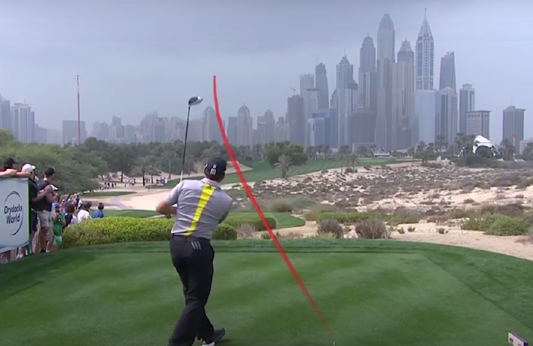
Figure 1: Source: https://azbigmedia.com/lifestyle/ball-tracking-technology-changes-way-fans-consume-practice-sport-of-golf/
Naive tracking will detect an object per frame without any regard for prior information. More sophisticated trackers will consider the previous frame as a starting point to their search space. However, even these trackers many need to initialize after a certain amount of time if their estimate drifts too far away from the object’s actual location.
Example of the importance of reliable tracking for driving assistance: https://youtu.be/NSDTZQdo6H8?t=898
Tracking with Optical Flow
Image motion can be described as complex changes in image intensity from one time to another, displaced by \(\delta\).
The displacement can be modeled as an affine motion field where the point is warped and translated by \(d\):
\[ \delta = D\mathbf{x} + \mathbf{x}, \]
where
\[ D = \begin{bmatrix} d_{xx} & d_{xy}\\ d_{yx} & d_{yy} \end{bmatrix}. \]
When comparing features between an image at \(t\) and \(t-1\), the feature centered at \(\mathbf{x}\) is transformed by
\[ \textbf{I}_{t}(A\mathbf{x} + \mathbf{d}) = \textbf{I}_{t-1}(\mathbf{x}). \]
Here, \(A = I_2 + D\), where \(I_2\) is the \(2 \times 2\) identity matrix. This addition will be explained later.
Smaller variations between frames are less reliable for parameter estimation, so a pure translational model is better in these cases. That is
\[ \delta = \mathbf{d}. \]
Computing Image Motion
Computing image motion then becomes a minimization problem.
\[ \epsilon = \int \int_{W} \big[\mathbf{I}_{t}(A\mathbf{x} + \mathbf{d}) - \mathbf{I}_{t-1}(\mathbf{x})\big]^2 w(\mathbf{x}) d\mathbf{x} \]
This is used in a minimization problem which will minimize the dissimilarity between the tracked features between frames. The point is weighted by a function \(w\) over a window \(W\).
Minimization of this error involves taking the derivative of \(\epsilon\) with respect to the unknowns in \(D\) and displacement vector \(\mathbf{d}\):
\begin{align*} \frac{1}{2}\frac{\partial \epsilon}{\partial D} &= \int \int_W \Big[\mathbf{I}_t(A\mathbf{x}+\mathbf{d}) - \mathbf{I}_{t-1}(\mathbf{x})\Big]\mathbf{g}\mathbf{x}^T w d\mathbf{x} = 0\\ \frac{1}{2}\frac{\partial \epsilon}{\partial \mathbf{d}} &= \int \int_W \Big[\mathbf{I}_t(A\mathbf{x}+\mathbf{d}) - \mathbf{I}_{t-1}(\mathbf{x})\Big]\mathbf{g} w d\mathbf{x} = 0\\ \end{align*}
where
\[ \mathbf{g} = \bigg(\frac{\partial \mathbf{I}_t}{\partial x}, \frac{\partial \mathbf{I}_t}{\partial y}\bigg)^T \]
is this spatial gradient of the image intensity. We have computed these image gradients before!
The transformation of a point from \(t\) to \(t+1\) is complex because of the potential rotation, scaling, and translation that can occur. Specifically, \(A\mathbf{x} + \mathbf{d}\) is a nonlinear transformation. To solve this with less friction, the term can be approximated.
To linearlize \(\mathbf{I}_{t}\), a Taylor series expansion of it can be used, taking just the linear term:
\[ \mathbf{I}_t(A\mathbf{x}+\mathbf{d}) = \mathbf{I}_t(\mathbf{x})+\mathbf{g}^T(\mathbf{u}), \]
where
\[ \mathbf{u} = D\mathbf{x}+\mathbf{d}. \]
The authors argue that this approximation is reasonable assuming the motion in the images is small.
Plugging this back into the derivatives above yields
\begin{align*} \int \int_W \mathbf{g}\mathbf{x}^T(\mathbf{g}^T\mathbf{u})w d\mathbf{x} &= \int \int_W \big[\mathbf{I}_{t-1}(\mathbf{x}) - \mathbf{I}_t\big]\mathbf{g}\mathbf{x}^T w d\mathbf{x}\\ \int \int_W \mathbf{g}(\mathbf{g}^T\mathbf{u})w d\mathbf{x} &= \int \int_W \big[\mathbf{I}_{t-1}(\mathbf{x}) - \mathbf{I}_t\big]\mathbf{g} w d\mathbf{x}\\ \end{align*}
This is solved iteratively, following the Newton method, starting with the following values at \(t=0\):
\begin{align*} D_0 &= I\\ \mathbf{d}_0 &= \mathbf{0}\\ \mathbf{I}_0 &= \mathbf{I}(\mathbf{x}). \end{align*}
At step \(i\) the values are updated to
\begin{align*} D_i\\ \mathbf{d}_i\\ \mathbf{I}_i &= \mathbf{I}_{i-1}(A_i \mathbf{x} + \mathbf{d}_i). \end{align*}
A More Compact Representation
At this point, the authors convert this representation into a more compact form in which the unknowns in \(D\) and the values of \(\mathbf{d}\) are separated from the function. We start with our current system of equations.
\begin{align*} \int \int_W \mathbf{g}\mathbf{x}^T(\mathbf{g}^T\mathbf{u})w d\mathbf{x} &= \int \int_W \big[\mathbf{I}_{t-1}(\mathbf{x}) - \mathbf{I}_t(\mathbf{x})\big]\mathbf{g}\mathbf{x}^T w d\mathbf{x}\\ \int \int_W \mathbf{g}(\mathbf{g}^T\mathbf{u})w d\mathbf{x} &= \int \int_W \big[\mathbf{I}_{t-1}(\mathbf{x}) - \mathbf{I}_t(\mathbf{x})\big]\mathbf{g} w d\mathbf{x}\\ \end{align*}
To achieve this, the Kronecker product is used. This is a generalization of the outer product from vectors to matrices. For two matrices \(A \in \mathbb{R}^{p \times q}\) and \(B \in \mathbf{R}^{m \times n}\), \(A \otimes B\) is a \(p \times q\) block matrix
\[ A \otimes B = \begin{bmatrix} a_{11}B & \cdots & a_{1q}\\ \vdots & \ddots & \vdots\\ a_{p1}B & \cdots & a_{pq}B \end{bmatrix}. \]
It has two particularly useful properties for this problem:
- \(A^T \otimes B^T = (A \otimes B)^T\)
- \(v(AXB) = (B^T \otimes A)v(X)\), where \(v\) is the vectorization operator.
Using this product and the properties just listed, we can extract the unknowns \(D\) and \(\mathbf{d}\) from the equations above.
First, note that \(\mathbf{g}^T \mathbf{u}\) appear in both of the equations. These can then be rewritten as follows.
\begin{align*} \mathbf{g}^T \mathbf{u} &= \mathbf{g}^T(D\mathbf{x} + \mathbf{d})\\ &= \mathbf{g}^T D \mathbf{x} + \mathbf{g}^T \mathbf{d}\\ &= v(\mathbf{g}^T D \mathbf{x}) + \mathbf{g}^T \mathbf{d} &\text{ vectorization }\\ &= (\mathbf{x}^T \otimes \mathbf{g}^T)v(D) + \mathbf{g}^T \mathbf{d} &\text{ property 2 }\\ &= (\mathbf{x} \otimes \mathbf{g})^T v(D) + \mathbf{g}^T \mathbf{d} &\text{ property 1 } \end{align*}
Likewise, the term \(\mathbf{g}\mathbf{x}^T\) that appears on the right side of the first equation in our set to solve can be written as
\begin{align*} v(\mathbf{g}\mathbf{x}^T) &= v(\mathbf{g}1\mathbf{x}^T)\\ &= \mathbf{x} \otimes \mathbf{g}. \end{align*}
Plugging this into the first equation to solve from above yields
\[ \int \int_W (\mathbf{x} \otimes \mathbf{g})((\mathbf{x} \otimes \mathbf{g})^T v(D) + \mathbf{g}^T\mathbf{d})w d\mathbf{x} = \int \int_W \big[\mathbf{I}_{t-1}(\mathbf{x}) - \mathbf{I}_t(\mathbf{x})\big](\mathbf{x} \otimes \mathbf{g}) w d\mathbf{x}. \]
Expanding these terms out produces
\begin{align*} \bigg(\int \int_W (\mathbf{x} \otimes \mathbf{g})(\mathbf{x} \otimes \mathbf{g})^T w d\mathbf{x}\bigg) v(D) + \bigg(\int \int_W (\mathbf{x} \otimes \mathbf{g}) \mathbf{g}^T w d\mathbf{x}\bigg) \mathbf{d}\\ = \int \int_W \big[\mathbf{I}_{t-1}(\mathbf{x}) - \mathbf{I}_t(\mathbf{x})\big](\mathbf{x} \otimes \mathbf{g}) w d\mathbf{x}. \end{align*}
The authors further simplify this equation using the following variables:
\begin{align*} U(\mathbf{x}) &= (\mathbf{x} \otimes \mathbf{g})(\mathbf{x} \otimes \mathbf{g})^T\\ V(\mathbf{x}) &= (\mathbf{x} \otimes \mathbf{g})\mathbf{g}^T\\ \mathbf{b}(\mathbf{x}) &= \big[\mathbf{I}_{t-1}(\mathbf{x}) - \mathbf{I}_{t}(\mathbf{x})\big]v(\mathbf{g}\mathbf{x}^T). \end{align*}
Then the above equation can be written as
\[ \bigg(\int \int_W U(\mathbf{x}) w d\mathbf{x}\bigg) v(D) + \bigg(\int \int_W V(\mathbf{x}) w d\mathbf{x}\bigg) \mathbf{d} = \int \int_W \mathbf{b}(\mathbf{x}) w d\mathbf{x}. \]
To write the second equation in a similar way, the authors introduce two additional variables
\begin{align*} Z(\mathbf{x}) &= \mathbf{g}\mathbf{g}^T\\ \mathbf{c}(\mathbf{x}) &= \big[\mathbf{I}_{t-1}(\mathbf{x}) - \mathbf{I}_t(\mathbf{x})\big]\mathbf{g}. \end{align*}
Then,
\[ \bigg(\int \int_W V^T(\mathbf{x}) w d\mathbf{x}\bigg) v(D) + \bigg(\int \int_W Z(\mathbf{x}) w d\mathbf{x}\bigg) \mathbf{d} = \int \int_W \mathbf{c}(\mathbf{x}) w d\mathbf{x}. \]
These equations can be written in a simple form: \(A\mathbf{x} + B\mathbf{y} = \mathbf{z}\). A symmetric block matrix \(T \in \mathbb{R}^{6 \times 6}\) is then introduced:
\begin{align*} T &= \int \int_W \begin{bmatrix} U & V\\ V^T & Z \end{bmatrix} w d\mathbf{x}\\ &= \int \int_W \begin{bmatrix} x^2g_x^2 & x^2 g_x g_y & x y g_x^2 & x y g_x g_y & x g_x^2 & x g_x g_y\\ x^2 g_x g_y & x^2 g_y^2 & x y g_x g_y & x y g_y^2 & x g_x g_y & x g_y^2\\ x y g_x^2 & x y g_x g_y & y^2 g_x^2 & y^2 g_x g_y & y g_x^2 & y g_x g_y\\ x y g_x g_y & x y g_y^2 & y^2 g_x g_y & y^2 g_y^2 & y g_x g_y & y g_y^2\\ x g_x^2 & x g_x g_y & y g_x^2 & y g_x g_y & g_x^2 & g_x g_y\\ x g_x g_y & x g_y^2 & y g_x g_y & y g_y^2 & g_x g_y & g_y^2 \end{bmatrix}w d \mathbf{x}. \end{align*}
Look very closely at \(Z\). Does that remind you of anything? Harris corner detection!
The unknowns are vectorized as
\[ \mathbf{z} = \begin{bmatrix} v(D)\\ \mathbf{d} \end{bmatrix}. \]
The product vector is defined as
\begin{align*} \mathbf{a} &= \int \int_W \begin{bmatrix} \mathbf{b}\\ \mathbf{c} \end{bmatrix} w d \mathbf{x}\\ &= \int \int_W \Big[\mathbf{I}_{t-1}(\mathbf{x}) - \mathbf{I}_t(\mathbf{x})\Big]\begin{bmatrix} x g_x\\ x g_y\\ y g_x\\ y g_y\\ g_x\\ g_y \end{bmatrix} w d \mathbf{x}. \end{align*}
Thus, the iterative solution requires solving the \(6 \times 6\) linear system
\[ T \mathbf{z} = \mathbf{a}. \]
Back to Computing Image Motion
With this more compact representation, the iterative solution is easier to achieve. The authors conveniently note that the deformation of the feature window between frames will be relatively small, so \(D\) could be set to 0 for tracking. This leads to the solution of a much smaller system for each time step:
\[ Z \mathbf{d} = \begin{bmatrix} g_x\\ g_y \end{bmatrix}. \]
Note that this is only true for small steps between frames. It is also important to measure the dissimilarity between the feature at the initial frame as it changes over time with the iterative estimates. If it changes too much, the dissimilarity will be high, indicating that it is no longer a reliable feature to track.
Picking the Best Feature
Shi and Tomasi posit that the best feature is one that can be tracked well.
“We can track a window from frame to frame if this system represents good measurements, and if it can be solved reliably.”
They analyze the basic equation \(Z \mathbf{d} = \mathbf{e}\), which is solved during tracking. If both eigenvalues of \(Z\) are large and do not differ by several orders of magnitude, the feature can be tracked reliably. That is, they accept a window if the eigenvalues of \(Z\) satisfy
\[ \min(\lambda_1, \lambda_2) > \lambda. \]
In practice, \(\lambda\) is determined by selecting a lower bound based on a region of uniform brightness in the image as well as an upper bound based on features such as corners. The selected value of \(\lambda\) is somewhere in between.
Measuring dissimilarity
To determine if a feature is still reliable over a longer time period, a measure of dissimilarity is used to measure the original feature versus its warped version at the current frame. Consider the sequence below over 21 frames.
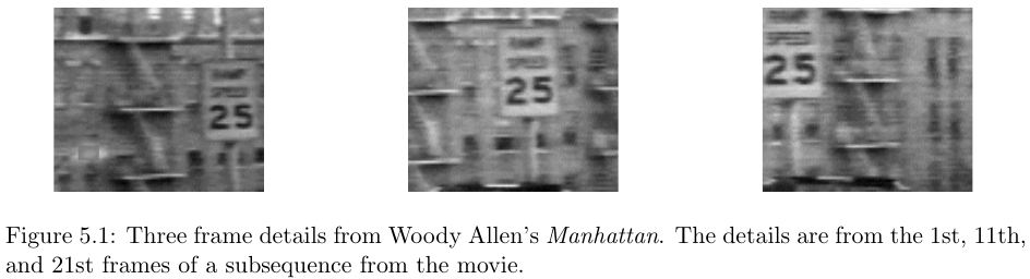
Figure 2: Source: Shi and Tomasi.
Their method successfully tracks the speed limit sign, as seen below.
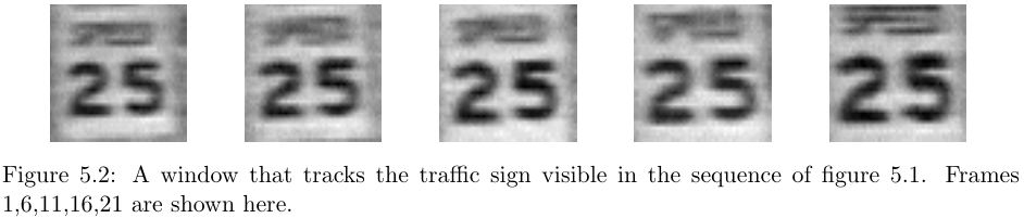
Figure 3: Source: Shi and Tomasi.
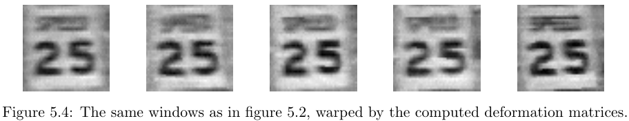
Figure 4: Source: Shi and Tomasi.
They note the importance of using an affine deformation to track reliable features. The figure below plots the dissimilarity using translation versus the deformation matrix over time.
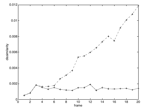
Figure 5: Dissimilarity over time using translation (dashed) versus affine (solid) (Shi and Tomasi).
They also present a case when the feature is lost to occlusion, thus the dissimilarity of both approaches increases greatly over time.
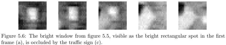
Figure 6: Source: Shi and Tomasi.
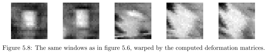
Figure 7: Source: Shi and Tomasi.
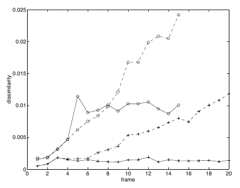
Figure 8: Sign tracking (plusses) versus window tracking (circles) (Shi and Tomasi).
Kalman Filters
A Kalman filter is a linear dynamic model that models conditional probabilities following normal distributions. It is an simple and effective model for tracking motion even in the presence of noise from measurements. Kalman filters keep an estimate of the state and can update their estimates based on the given observations.
\(\mathbf{X}_i\) - State of object at step \(i\)
\(\mathbf{Y}_i\) - Measurement at step \(i\)
There are two primary tasks to deal with, the real-time tracking task and the offline smoothing task. We are more interested in the tracking task, so we will focus on that.
Tracking task: \(P(X_k|Y_0, \dots, Y_k)\)
Smoothing task: \(P(X_k|X_0, \dots, Y_n)\)
Assumptions:
- \(P(Y_k|X_0, \dots, X_N, Y_0, \dots, Y_N) = P(Y_k|X_k)\)
- \(P(X_k|X_0, \dots, X_{k-1}) = P(X_k|X_{k-1})\)
Prediction Task
When tracking an object, we use the model to first predict a state and then update its current parameters given some measurement. We want to predict the state given measurements: \(P(\mathbf{X}_i|\mathbf{Y}_0 = \mathbf{y}_0, \dots, \mathbf{Y}_{k-1}=\mathbf{y}_{k-1})\).
Given the previous observations up to \(k-1\), what is our model’s estimate of the current state? This can help establish a search location if we were looking to narrow our detection algorithm.
Correction
\(P(\mathbf{X}_i|\mathbf{Y}_0 = \mathbf{y}_0, \dots, \mathbf{Y}_{i}=\mathbf{y}_{i})\) is the cur rent distribution. This is the estimate given the actual observation at \(i\). Note that this observation could be given from a noisy measurement.
Linear Dynamics
Assuming linear models, the problem becomes much simpler. We can model the observations and state using normal distributions.
\[ \mathbf{x} \sim \mathcal{N}(\mathbf{\mu}, \Sigma) \]
The measurements themselves can be modeled as
\[ \mathbf{y}_i \sim \mathcal{N}(\mathcal{B}_i \mathbf{x}_i, \Sigma_i), \]
where \(i\) is the current step.
In other words, our model does not know the true position and velocity of objects at all times. If this were the case, tracking would be a trivial pursuit. This uncertainty is captured using Gaussian distributions. This is a reasonable assumption to make in many cases. It becomes more complex if we think about acceleration, but we could always model that as well.
By the way, position and velocity are correlated. If the velocity of the current object is 0, you would probably bet that its position in the next frame will be the same. A covariance matrix tracks this correlation between the variables. The problem is starting to take shape. We have input and observation variables as well as a covariance matrix that defines the relationship between our position and velocity.
For the future, the model will be represented as
\begin{align*} \mathbf{x}_i &\sim \mathcal{N}(\mathcal{D}_i \mathbf{x}_{i-1}; \Sigma_{d_i})\\ \mathbf{y}_i &\sim \mathcal{N}(\mathcal{M}_i \mathbf{x}_i; \Sigma_{m_i}). \end{align*}
The mean parameter in both of these look a little strange; we usually see \(\mu\) here. The matrix \(\mathcal{D}_i\), for example, transforms the center of the Gaussian to an updated location. Consider a bird flying through the sky in a relatively straight pattern. Of course, there will be some variation due to external factors or the bird’s desire to move about. Modeling this motion with a Gaussian centered at the mean \(\mathbf{x}_{i-1}\) would be insufficient.
For one, the likelihood that the bird would instantly change course is physically impossible. It could start to turn, but the resolution of our update steps would track this over a sequence of frames. Instead, we transform the value \(\mathbf{x}_{i-1}\) based on our current perception of the bird’s movement dynamics. This translates the Gaussian to a new location. It also has the possibility of changing its shape.
For covering the algorithm, we will use notation following Forsyth and Ponce. \(\bar{\mathbf{x}}_i^-\) is the mean of \(P(\mathbf{x}_i|y_0, \dots, y_{i-1})\) and \(\bar{\mathbf{x}}_i^+\) is the mean of \(P(\mathbf{x}_i|y_0, \dots, y_{i})\). \(\Sigma_i^-\) and \(\Sigma_i^+\) are the covariances of those distributions.
However, by making a convenient assumption about the observation model, we will mainly need to focus on the state model. That is, the matrix \(\mathcal{M}_i\) is defined so that the mean is simply the state position at step \(i\).
What does our state represent?
In a simple model, \(\mathbf{x} = \begin{bmatrix}p_x\\p_y\\v_x\\v_y\end{bmatrix}\). That is the 2D position and velocity of the object being tracked. The corresponding covariance matrix is \(\mathbf{x}\mathbf{x}^T\).
How do we predict the position and velocity of the next time step?
\begin{align*} \mathbf{p}_i &= \mathbf{p}_{i-1} + \Delta t \mathbf{v}_{i-1}\\ \mathbf{v}_i &= \mathbf{v}_{i-1} \end{align*}
This is making a simple, yet surprisingly effective, assumption that the velocity is constant. We can write this as a matrix vector product:
\[ \mathbf{x}_i = \begin{bmatrix} 1 & 0 & \Delta t & 0\\ 0 & 1 & 0 & \Delta t\\ 0 & 0 & 1 & 0\\ 0 & 0 & 0 & 1 \end{bmatrix} \mathbf{x}_{i-1} \]
Compactly, the prediction for step \(t\) is \(\bar{\mathbf{x}}_i^- = \mathcal{D}_i \bar{\mathbf{x}}_{i-1}^+\).
Since we updated every point \(\mathbf{x}_{i-1}\), we also need to make a prediction about the covariance matrix. This is also achieved by multiplying every point by \(\mathcal{D}_i\)
\[ \Sigma_{i}^- = \mathcal{D}_i\Sigma_{i-1}^+\mathcal{D}_i^T \]
What if we want to add additional knowledge like acceleration?
Our position prediction then follows
\begin{align*} \mathbf{p}_i &= \mathbf{p}_{i-1} + \Delta t \mathbf{v}_{i-1} + \frac{1}{2} \Delta t^2 \mathbf{a}_{i-1}\\ \mathbf{v}_i &= \mathbf{v}_{i-1} + \Delta t \mathbf{a}_{i-1} \end{align*}
We can simplify this and assume constant acceleration, then \(\mathbf{a}_i = \mathbf{a}_{i-1}\). The resulting update equation for \(\mathbf{x}_k\) becomes
\[ \mathbf{x}_i = \begin{bmatrix} 1 & 0 & \Delta t & 0 & \frac{1}{2}\Delta t^2 \mathbf{a} & 0\\ 0 & 1 & 0 & \Delta t & 0 & \frac{1}{2}\Delta t^2 \mathbf{a}\\ 0 & 0 & 1 & 0 & \Delta t & 0\\ 0 & 0 & 0 & 1 & 0 & \Delta t\\ 0 & 0 & 0 & 0 & 1 & 0\\ 0 & 0 & 0 & 0 & 0 & 1\\ \end{bmatrix} \mathbf{x}_{i-1} \]
However, if something like acceleration is a known control factor in our system, then it does not need to be part of the state. In this case, we could separate the update vector into
\[ \mathbf{x}_i = \mathcal{D}_i\mathbf{x}_{i-1} + B_i \mathbf{u}_{i}, \]
where \(B_i\) is the control matrix and \(\mathbf{u}_i\) is the control vector.
One last consideration is that of uncertainty due to factors outside of our system. This can also be modeled using a Gaussian with zero mean and covariance \(\Sigma_d\):
\[ \xi_i \sim \mathcal{N}(\mathbf{0}, \Sigma_{d_i}). \]
With this added noise, the prediction step becomes
\begin{align*} \bar{\mathbf{x}}_i^- &= \mathcal{D}_i\bar{\mathbf{x}}_{i-1}^+ + B_i \mathbf{u}_i\\ \Sigma_i^- &= \mathcal{D}_i \Sigma_{i-1}^+\mathcal{D}_i^T + \xi_i. \end{align*}
In words, \(\bar{\mathbf{x}}_i^-\) is the prediction of our current state based on the previous best estimate with an added correction term based on known factors (acceleration). \(\Sigma_i^-\) is the updated uncertainty based on the old uncertainty with added Gaussian noise to reflect unknown factors.
Making Corrections
As we are tracking an object, we may have some way of getting measurements. This could be through an object detector or other physical sensor. The new measurement can refine our current set of parameters. Kalman filters work well even if the measurement is noisy.
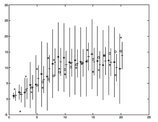
Figure 9: 1D Kalman Filter. Source: Forsyth and Ponce
In the figure above, the initial prediction has a large amount of uncertainty. After updating with the current measurement, the uncertainty is reduced.
The goal here is to reconcile the uncertainty of our predicted state with the uncertainty of the measurement. That is, we want to know the distribution over the union of these two distributions. This is achieved by multiplying the Gaussians together.
\[ \mathcal{N}(\bar{\mathbf{x}}_i^+, \Sigma_i^+) = \mathcal{N}(\bar{\mathbf{x}}_i^-, \Sigma_i^-) * \mathcal{N}(\mathbf{y}_i, \Sigma_{m_i}) \]
Solving for \(\bar{\mathbf{x}}_i^+\) and \(\Sigma_i^+\) yields
\begin{align*} \bar{\mathbf{x}}_i^+ &= \bar{\mathbf{x}}_i^- + \mathcal{K}_i(\mathbf{y}_i - \mathcal{M}_i \bar{\mathbf{x}}_i^-)\\ \Sigma_i^+ &= \Sigma_i^- - \mathcal{K}_i \mathcal{M}_i \Sigma_i^-, \end{align*}
where
\[ \mathcal{K}_i = \Sigma_i^- \mathcal{M}_i^T(\mathcal{M}_i \Sigma_i^- \mathcal{M}_i^T + \Sigma_{m_i})^{-1}. \]
\(\mathcal{K}_i\) is called the Kalman gain.
Let’s summarize the prediction and correction steps
We have a state distribution with mean and variance
\begin{align*} \bar{\mathbf{x}}_i^- &= \mathcal{D}_i\bar{\mathbf{x}}_{i-1}^+ + B_i \mathbf{u}_i\\ \Sigma_i^- &= \mathcal{D}_i \Sigma_{i-1}^+\mathcal{D}_i^T + \xi_i \end{align*}
as well as an observation distribution with mean and variance \(\mathbf{y}_i\) and \(\Sigma_{m_i}\).
The predictions are then refined by the observations via the following equations.
\begin{align*} \bar{\mathbf{x}}_i^+ &= \bar{\mathbf{x}}_i^- + \mathcal{K}_i(\mathbf{y}_i - \mathcal{M}_i \bar{\mathbf{x}}_i^-)\\ \Sigma_i^+ &= \Sigma_i^- - \mathcal{K}_i \mathcal{M}_i \Sigma_i^-, \end{align*}
where
\[ \mathcal{K}_i = \Sigma_i^- \mathcal{M}_i^T(\mathcal{M}_i \Sigma_i^- \mathcal{M}_i^T + \Sigma_{m_i})^{-1}. \]