Transformers for Computer Vision
Vision Transformer (ViT) (Dosovitskiy et al. 2021)
The original Vision Transformer (ViT) was published by Google Brain with a simple objective: apply the Transformer architecture to images, adding as few modifications necessary. When trained on ImageNet, as was standard practice, the performance of ViT does not match models like ResNet. However, scaling up to hundreds of millions results in a better performing model.
This point is highlighted in the introduction of the paper, but isn’t that something that should be expected? If anything, that result simply implies that CNNs are more parameter efficient than ViT. Seeing as this was one of the first adaptations of this architecture to vision, some slack should be given.
The Model
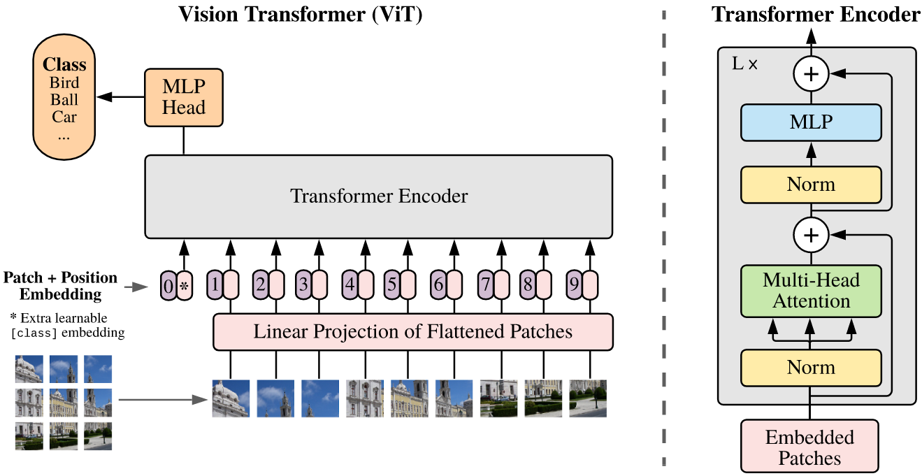
The first challenge is to figure out how to pass an image as input to a Transformer. In the original paper, the input is a sequence of text embeddings. If we get creative, there are a number of ways we could break up an image.
-
Split the image into individual patches.
This is what the ViT paper does. Each patch is flattened to a \(P^2 \cdot C\) vector, where \(P\) is the size of each square patch. Another reason the image is split into patches is to reduce the size of weight matrix of the attention layers. Using the entire image as a single input would be prohibitive.
-
Process individual image patches through a CNN.
This approach has been tried with some success, but isn’t the preferred approach for this paper. The goal, after all, is to conform as closely as possible to the original architecture. One could really run away with this idea. Processing each patch independently through a CNN woud be cumbersome and most likely result in a loss of spatial information. The original image could be processed through a CNN before splitting up the feature maps. This is discussed in the ViT paper as the hybrid approach.
-
Use output feature maps from a CNN.
This approach relates somewhat to number 2. Given a series of output feature maps \(X \in \mathbb{R}^{C \times H \times W}\), pass each feature map as its own patch a la the author’s approach. The feature maps would not be related spatially, but through the channels.
Taking the first approach, the patches are projected to a \(D\) dimensional vector the authors refer to as patch embeddings.
Transformer Encoder
The encoder is where the architecture models vision. The attention blocks effectively learn relationships between different patches. It facilitates the model’s ability to make sense of how different features are pieced together.
After the attention layer comes an MLP layer. The purpose of this is to refine the aggregate features given the context it just gathered from the attention block.
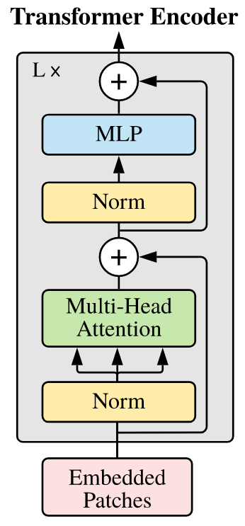
Figure 1: Encoder block (Dosovitskiy et al. 2021).
Learnable Embeddings
As is done in BERT, the author’s attach a [class] token to the sequence of embedded patches. The purpose of this is to aggregate information from all the patches via self-attention. The output is a learned global representation of the input image. This output vector is then passed through a classification head.
Since the encoder is a sequence-to-sequence model, each patch produces an output. The global context is the only piece that is used for tasks such as classification since it encodes information from all other patches.
Position Embeddings
Two immediate choices for position embeddings are either 1D or 2D-aware. The embeddings themselves are learnable. The authors opt for 1D learnable embeddings due to their simplicity and the fact that there was no noticeable performance difference when using 2D-aware embeddings.
The position embeddings are crucial for ViT since the each patch is represented as an embedding. While each patch embedding does retain locality, the relationship between the patches is not preserved. This relationship is learned via position embeddings. Basically, the inductive biases that CNNs have must be learned in a ViT.
Using Higher Resolutions
When using higher resolution input, the patch size is kept the same. This means that the sequence length is increases to accommodate the larger number of patches. Although the input to the Transformer can handle an abitrary sequence length, the position embeddings learned at one resolution are useless when fine-tuned on another.
Evaluations
Most of the information in the original ViT paper is dedicated to experiments. The model itself is a simple adaptation. The primary goal then is to evaluate its characteristics and how it performs compared to CNNs.
Key Results
- ViT achieves better downstream accuracy than SOTA ResNet-based approaches using JFT-300M for pre-training.
- ViT requires fewer computational resources.
- CNN models perform better when pre-trained on smaller datasets compared to ViT, but ViT surpasses them when using very large datasets. This is attributed to the inductive bias that is built into the CNN architecture.
Properties
The principal components of the patch embeddings resemble features learned in the early layers of a CNN. The authors did not investigate whether ViT builds a hierarchy of features similar to CNNs. However, later work confirmed that the features learned at each layer of a ViT progress in a similar manner (Ghiasi et al. 2022).

Figure 2: The progression for visualized features of ViT B-32 (Ghiasi et al. 2022).
The position embeddings were also analyzed and the authors found that patches that are grouped together tend to have similar embeddings. The fact that these embeddings learned 2D relationships gives weight to the argument that hand-crafted 2D-aware embeddings do not perform any better.
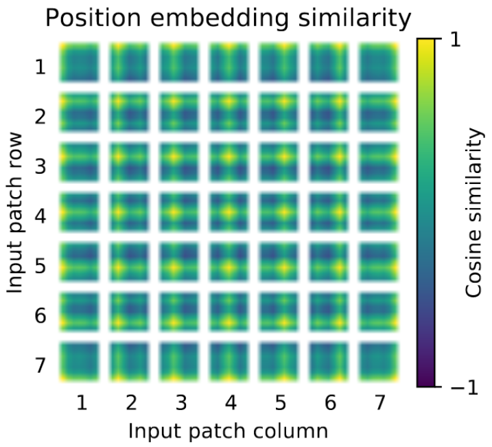
Figure 3: Position embedding similarity (Dosovitskiy et al. 2021).
The self-attention mechanisms in ViT attend to information globally across the entire image. The authors verify this by computing the average distance in image space across which the information is used. The distance varies between the different attention heads. Some heads attend to most of the detail in the lowest layer. This suggests that global information is used by the model since it attends across the representations in these early layers. Other heads have a smaller attention distance, suggesting they are focusing on local information.
In later work, it was discovered that earlier layers will not learn to attend locally given smaller pre-training datasets (Raghu et al. 2022).
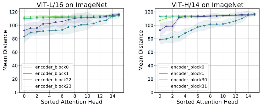
Figure 4: With less training data, lower attention layers do not learn to attend locally (Raghu et al. 2022).
One interesting result with respect to the hybrid models it that they do not observe as much local attention. This is most likely because local spatial relationships are captured by the early layers of a CNN. In hybrid models, the Transformer received processed feature maps from CNNs.
Self-Supervision
Self-supervised pre-training is one of the key ingredients to training LLMs (Radford et al. 2018). The authors of ViT experiment with self-supervised pre-training by masking out different patches and having the model predict the masked regions, similar to BERT (Devlin et al. 2019). With self-supervised pre-training, ViT-B/16 achieves 79.9% accuracy on ImageNet, 2% higher compared to training from scratch.
Swin Transformer (Liu et al. 2021)
- Introduces a general backbone for computer vision tasks.
- Builds a hierarchical transformer to allow for non-overlapping windows.
- Can be used for classification, object detection, and instance segmentation.
- Has linear complexity compared to input image size.
Architecture
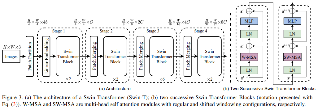
Figure 5: Swin-T architecture (Liu et al. 2021).
- Split input into patches similar to other ViT approaches.
- Pass through Swin blocks, maintaining \((\frac{H}{4} \times \frac{W}{4})\) tokens.
- Patches are merged by concatenating the features of each group of \(2 \times 2\) neighboring patches. They are then projected linearly to a lower dimensionality.
- A Swin Transformer block goes through an initial attention block followed by a shifted window attention block. The initial attention block focuses on building local understanding. Shifting the windows permits attention across patches from different windows.
- This continues for several layers as defined by the model size.
Image Classification
For classification, global average pooling is applied to the output feature map. This is then fed into a linear classifier.
Object Detection and Segmentation
Swin is used as a backbone for object detection and segmentation. For object detection, Mask R-CNN components are used. For semantic segmentation, UperNet and FPN decoders are employed.
