Heapsort
The lecture slides for these notes are available here.
- Running time is \(O(n \lg n)\).
- Sorts in place, only a constant number of elements needed in addition to the input.
- Manages data with a heap.
A binary heap can be represented as a binary tree, but is stored as an array. The root is the first element of the array. The left subnode for the element at index \(i\) is located at \(2i\) and the right subnode is located at \(2i + 1\). This assumes a 1-based indexing.
Using 0-based indexing, we can use \(2i + 1\) for the left and \(2i + 2\) for the right. The parent could be accessed via \(\lfloor \frac{i-1}{2} \rfloor\).
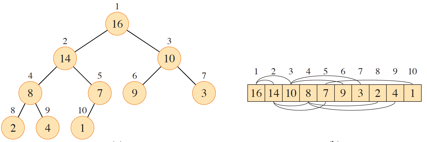
Figure 1: A binary tree as a heap with its array representation (Cormen et al. 2022).
Heaps come in two flavors: max-heaps and min-heaps. They can be identified by satisfying a heap property.
- max-heap property: \(A[parent(i)] \geq A[i]\)
- min-heap property: \(A[parent(i)] \leq A[i]\)
These properties imply that the root is the largest element in a max-heap and the smallest element in a min-heap.
When it comes to heapsort, a max-heap is used. Min-heaps are used in priority queues. These notes will cover both.
Maintaining the Heap Property
When using heapsort, the heap should always satisfy the max-heap property. This relies on a procedure called max_heapify. This function assumes that the root element may violate the max-heap property, but the subtrees rooted by its subnodes are valid max-heaps. The function then swaps nodes down the tree until the misplaced element is in the correct position.
def max_heapify(A, i, heap_size):
    l = left(i)
    r = right(i)
    largest = i
    if l < heap_size and A[l] > A[i]:
        largest = l
    if r < heap_size and A[r] > A[largest]:
        largest = r
    if largest != i:
        A[i], A[largest] = A[largest], A[i]
        max_heapify(A, largest, heap_size)
Analysis of Max Heapify
Given that max_heapify is a recursive function, we can analyze it with a recurrence. The driving function in this case would be the fix up that happens between the current node and its two subnodes, which is a constant time operation. The recurrence is based on how many elements are in the subheap rooted at the current node.
In the worst case of a binary tree, the last level of the tree is half full. That means that the left subtree has height \(h + 1\) compared to the right subtree’s height of \(h\). For a tree of size \(n\), the left subtree has \(2^{h+2}-1\) nodes and the right subtree has \(2^{h+1}-1\) nodes. This is based on a geometric series.
We now have that the number of nodes in the tree is equal to \(1 + (2^{h+2}-1) + (2^{h+1}-1)\).
\begin{align*} n &= 1 + 2^{h+2} - 1 + 2^{h+1} - 1 \\ n &= 2^{h+2} + 2^{h+1} - 1 \\ n &= 2^{h+1}(2 + 1) - 1 \\ n &= 3 \cdot 2^{h+1} - 1 \end{align*}
This implies that \(2^{h+1} = \frac{n+1}{3}\). That means that, in the worst case, the left subtree would have \(2^{h+2} - 1 = \frac{2(n+1)}{3} - 1\) nodes which is bounded by \(\frac{2n}{3}\). Thus, the recurrence for the worst case of max_heapify is \(T(n) = T(\frac{2n}{3}) + O(1)\).
Building the Heap
Given an array of elements, how do we build the heap in the first place? The solution is to build it using a bottom-up approach from the leaves. The elements from \(\lfloor \frac{n}{2} \rfloor + 1\) to \(n\) are all leaves. This means that they are all 1-element heaps. We can then run max_heapify on the remaining elements to build the heap.
def build_max_heap(A):
    heap_size = len(A)
    for i in range(len(A) // 2, -1, -1):
        max_heapify(A, i, heap_size)
Why does this work?
Each node starting at \(\lfloor \frac{n}{2} \rfloor + 1\) is the root of a 1-element heap. The subnodes, which are to the right of node \(\lfloor \frac{n}{2} \rfloor\), are roots of their own max-heaps. The procedure loops down to the first node until all sub-heaps have been max-heapified.
The figure below is from (Cormen et al. 2022) and shows the process of building a max-heap from an array.
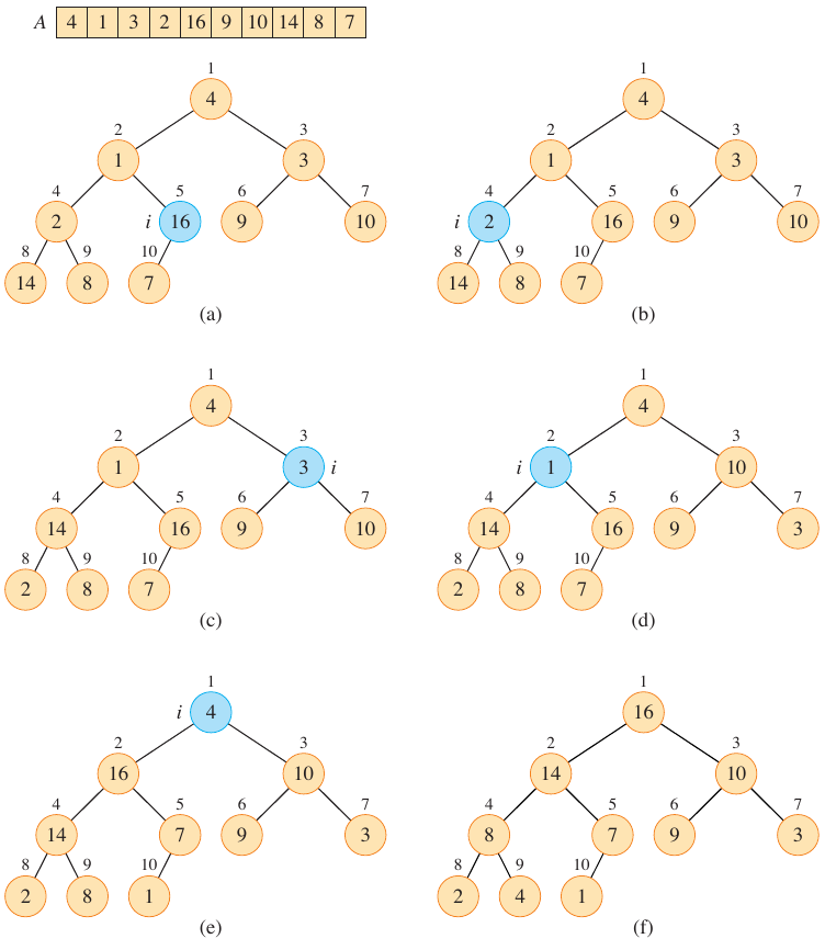
Figure 2: Building a max-heap from an array (Cormen et al. 2022).
Analysis of Build Max Heap
A general analysis is fairly straightforward considering that the call to max_heapify is \(O(\lg n)\). The loop in build_max_heap runs \(O(n)\) times. This means that the overall running time is \(O(n \lg n)\). A more careful analysis can be done by considering the height of the tree and the number of nodes at each level.
A heap of \(n\) elements has height \(\lfloor \lg n \rfloor\) Each call to max_heapify can also be viewed in terms of the height of the tree \(h\), so the upper bound is \(O(h)\). This bounds build_max_heap at \(\sum_{h=0}^{\lfloor \lg n \rfloor} \lceil \frac{n}{2^{h+1}} \rceil ch\). When \(h = 0\), the first term \(\lceil \frac{n}{2^{h+1}} \rceil = \lceil \frac{n}{2} \rceil\). When \(h = \lfloor \lg n \rfloor\), \(\lceil \frac{n}{2^{h+1}} \rceil = 1\). Thus, \(\lceil \frac{n}{2^{h+1}} \rceil \geq \frac{1}{2}\) for \(0 \leq h \leq \lfloor \lg n \rfloor\).
Let \(x = \frac{n}{2^{h+1}}\). Since \(x \geq \frac{1}{2}\), we have that \(\lceil x \rceil \leq 2x\). This means that \(\lceil \frac{n}{2^{h+1}} \rceil \leq \frac{2n}{2^{h+1}} = \frac{n}{2^h}\). An upper bound can now be derived.
\begin{align*} \sum_{h=0}^{\lfloor \lg n \rfloor} \lceil \frac{n}{2^{h+1}} \rceil ch &\leq \sum_{h=0}^{\lfloor \lg n \rfloor} \frac{n}{2^h} ch \\ &= cn \sum_{h=0}^{\lfloor \lg n \rfloor} \frac{h}{2^h} \\ &\leq cn \sum_{h=0}^{\infty} \frac{h}{2^h} \\ &\leq cn \cdot \frac{1 / 2}{(1 - 1/2)^2}\quad \text{(See CRLS for details)} \\ &= O(n) \end{align*}
Thus, a heap can be constructed in linear time. This is independent on whether the original data is already sorted.
Heapsort
We now have all of the components necessary to implement heapsort. The algorithm is as follows:
def heapsort(A):
    build_max_heap(A)
    heap_size = len(A)
    for i in range(len(A) - 1, 0, -1):
        A[0], A[i] = A[i], A[0]
        heap_size -= 1
        max_heapify(A, 0, heap_size)
It starts by building a max-heap on the input array. As seen in the previous section, this is done in linear time. From there, it’s a matter of taking the root element out of the heap and then running max_heapify to maintain the max-heap property. This is done \(n-1\) times, so the overall running time is \(O(n \lg n)\).
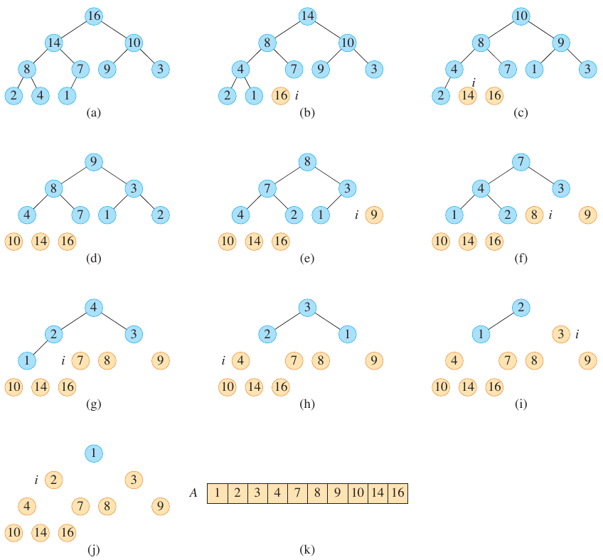
Figure 3: Heapsort in action (Cormen et al. 2022).
Heapsort is visualized in the figure above, starting with a constructed max-heap in (a) (Cormen et al. 2022).
Questions
- What is the running time of heapsort given an array that is already sorted in ascending order?
- What is the running time of heapsort given an array that is already sorted in descending order?