Kernels
Slides for these notes can be found here. Check out MLST’s episode on Kernels.
Introduction
Notebook link: https://github.com/ajdillhoff/CSE6363/blob/main/svm/kernels.ipynb
Parametric models use training data to estimate a set of parameters that can then be used to perform inference on new data. An alternative approach uses nonparametric methods, meaning the function is estimated directly from the data instead of optimizing a set of parameters.
One possible downside to such an approach is that it becomes less efficient as the amount of training data increases. Additionally, the transformation into a feature space such that the data becomes linearly separable may be intractable. Consider sequential data such as text or audio. If each sample has a variable number of features, how do we account for this using standard linear models with a fixed number of parameters?
The situations described above can be overcome through the use of the kernel trick. We will see that, by computing a measure of similarity between samples in the feature space, we do not need to directly transform each individual sample to that space.
A kernel function is defined as
\[ k(\mathbf{x}, \mathbf{x}’) = \phi(\mathbf{x})^T \phi(\mathbf{x}’), \]
where \(\phi\) is some function which transforms the input to a feature space.
Methods that require part or all of the training data to make prediction will benefit from using kernel representations, especially when using high dimensional data. Instead of transforming the data into a high dimensional space which may be computationally intractable, a measure of similarity via the inner product is used. The inner product is not the projection into some space. Instead, it represents the outcome of that projection.
If the input vector takes on the form of scalar products, it can be represented as a kernel function.
Dual Representation
The key to taking advantage of the kernel trick relies on reformulating our linear model into a dual representation. In this form, we will establish a dependence on the kernel function.
The following derivation of the dual representation for linear regression follows (Bishop). Consider the least squares loss with \(L2\) regularization, as we discussed with Linear Regression.
\[ J(\mathbf{w}) = \frac{1}{2}\sum_{i=1}^n(\mathbf{w}^T\phi(\mathbf{x}_i) - y_i)^2 + \frac{\lambda}{2} \mathbf{w}^T \mathbf{w} \]
Here, \(\phi\) is a basis function that transforms the input. This could also be a simple identity function in which \(\phi(\mathbf{x}) = \mathbf{x}\). To solve for \(\mathbf{w}\), we take the gradient of \(J(\mathbf{w})\) with respect to \(\mathbf{w}\) and set it to 0.
\begin{align*} \nabla_{\mathbf{w}}J(\mathbf{w}) &= \sum_{i=1}^n(\mathbf{w}^T\phi(\mathbf{x}_i) - y_i)\phi(\mathbf{x}_i) + \lambda \mathbf{w}\\ \implies \mathbf{w} &= -\frac{1}{\lambda}\sum_{i=1}^n(\mathbf{w}^T\phi(\mathbf{x}_i) - y_i)\phi(\mathbf{x}_i) \end{align*}
We can formulate this as a matrix-vector product by letting
\begin{equation*} \mathbf{\Phi} = \begin{bmatrix} \phi(\mathbf{x}_1)^T\\ \vdots \\ \phi(\mathbf{x}_n)^T\\ \end{bmatrix} \text{ and } a_{i} = -\frac{1}{\lambda}(\mathbf{w}^T\phi(\mathbf{x}_i) - y_i). \end{equation*}
Then, \(\mathbf{w} = \mathbf{\Phi}^T\mathbf{a}\), where \(\mathbf{a} = [a_1, \dots, a_n]^T\).
The dual representation is derived by reformulating \(J(\mathbf{w})\) in terms of \(\mathbf{a}\).
\begin{equation*} J(\mathbf{a}) = \frac{1}{2}\mathbf{a}^T\mathbf{\Phi}\mathbf{\Phi}^T\mathbf{\Phi}\mathbf{\Phi}^T\mathbf{a} - \mathbf{a}^T\mathbf{\Phi}\mathbf{\Phi}^T\mathbf{y} + \frac{1}{2}\mathbf{y}^T\mathbf{y} + \frac{\lambda}{2} \mathbf{a}^T\mathbf{\Phi}\mathbf{\Phi}^T\mathbf{a}, \end{equation*}
where \(\mathbf{y} = [y_1, \dots, y_n]\).
Looking at the products \(\mathbf{\Phi}\mathbf{\Phi}^T\), we see that these relate to our original kernel form: \(\phi(\mathbf{x}_i)^T\phi(\mathbf{x}_j)\). This product defines a Gram matrix \(\mathbf{K} = \mathbf{\Phi}\mathbf{\Phi}^T\) whose elements are \(k(\mathbf{x}_i, \mathbf{x}_j)\). Thus, we can rewrite \(J(\mathbf{a})\) as
\begin{equation*} J(\mathbf{a}) = \frac{1}{2}\mathbf{a}^T\mathbf{K}\mathbf{K}\mathbf{a} - \mathbf{a}^T\mathbf{K}\mathbf{y} + \frac{1}{2}\mathbf{y}^T\mathbf{y} + \frac{\lambda}{2}\mathbf{a}^T\mathbf{K}\mathbf{a}. \end{equation*}
Solving for \(\mathbf{a}\) can be done by computing the gradient of \(J(\mathbf{a})\) with respect to \(\mathbf{a}\) and setting the result to 0.
\begin{align*} \nabla_\mathbf{a}J(\mathbf{a}) = \mathbf{K}\mathbf{K}\mathbf{a} - \mathbf{K}\mathbf{y} + \lambda \mathbf{K}\mathbf{a} &= 0\\ \mathbf{K}\mathbf{a} + \lambda I\mathbf{a} - \mathbf{y} &= 0\\ (\mathbf{K} + \lambda I)\mathbf{a} &= \mathbf{y}\\ \mathbf{a} &= (\mathbf{K} + \lambda I)^{-1} \mathbf{y}. \end{align*}
With \(\mathbf{a}\) solved, we can complete the dual representation of our original linear regression model. Recall that
\begin{equation*} h(\mathbf{x}; \mathbf{w}) = \mathbf{w}^T\phi(\mathbf{x}). \end{equation*}
If we substitute \(\mathbf{w} = \mathbf{\Phi}^T\mathbf{a}\), we get
\begin{align*} f(\mathbf{x};\mathbf{a}) &= \mathbf{a}^T\mathbf{\Phi}\phi(\mathbf{x})\\ &= \Big[(\mathbf{K} + \lambda I)^{-1}\mathbf{y})\Big]^T\mathbf{\Phi}\phi(\mathbf{x}). \end{align*}
Again, the kernel form is apparent in the product \(\mathbf{\Phi}\phi(\mathbf{x})\). If we let \(k_i(\mathbf{x}) = k(\mathbf{x}_i,\mathbf{x})\) and
\begin{equation*} \mathbf{k}(\mathbf{x}) = \begin{bmatrix} k_1(\mathbf{x})\\ \vdots \\ k_n(\mathbf{x}) \end{bmatrix}, \end{equation*}
we can write the dual representation of our linear regression model as
\begin{equation*} f(\mathbf{x}) = \mathbf{k}(\mathbf{x})^T(\mathbf{K} + \lambda \mathbf{I})^{-1}\mathbf{y}. \end{equation*}
Relating Back to the Original Formulation
In this dual formulation, the solution for \(\mathbf{a}\) can be expressed as a linear combination of elements \(\phi(\mathbf{x})\). From above, we see that
\[ a_i = -\frac{1}{\lambda}\big(\mathbf{w}^T\phi(\mathbf{x}_i) - y_i\big). \]
Expanding this into individual coefficients yields
\begin{align*} a_i &= -\frac{1}{\lambda}\big(w_1\phi_1(\mathbf{x}_i) + \cdots + w_m \phi_m(\mathbf{x}_i) - y_i\big)\\ &= -\frac{w_1}{\lambda}\phi_1(\mathbf{x}_i) - \cdots - \frac{w_m}{\lambda} \phi_m(\mathbf{x}_i) + \frac{y_i}{\lambda}. \end{align*}
We are close, but we still need to do something about the term \(\frac{y_i}{\lambda}\). For this, we can multiply both sides of our equation by a convenient 1. That is, we multiply by
\[ \frac{\phi_1(\mathbf{x}_i) + \cdots + \phi_m(\mathbf{x}_i)}{\phi_1(\mathbf{x}_i) + \cdots + \phi_m(\mathbf{x}_i)}. \]
By doing this and grouping the \(\phi_j\) terms, we get
\begin{align*} &\Big(\frac{y_i}{\lambda}\cdot \frac{1}{\phi_1(\mathbf{x}_i) + \cdots + \phi_m(\mathbf{x}_i)} - \frac{w_1}{\lambda}\Big)\phi_1(\mathbf{x}_i) + \cdots\\ &+ \Big(\frac{y_i}{\lambda}\cdot \frac{1}{\phi_1(\mathbf{x}_i) + \cdots + \phi_m(\mathbf{x}_i)} - \frac{w_m}{\lambda}\Big)\phi_m(\mathbf{x}_i). \end{align*}
We can simplify this by introducing a term
\[ c_i = \frac{y_i}{\lambda}\cdot \frac{1}{\phi_1(\mathbf{x}_i) + \cdots + \phi_m(\mathbf{x}_i)}. \]
Then the solution can be rewritten as
\[ \Big(c_i - \frac{w_1}{\lambda}\Big)\phi_1(\mathbf{x}_i) + \cdots + \Big(c_i - \frac{w_m}{\lambda}\Big)\phi_m(\mathbf{x}_i). \]
With this, we can step backwards using intermediate results in the previous section to get back to the original formulation of our linear regression model.
Types of Kernels
There are several types of kernels that can be used to transform the input data depending on the problem. The simplest kernel is the identity kernel:
\[ k(\mathbf{x}, \mathbf{x’}) = \mathbf{x}^T \mathbf{x’}. \]
Polynomial Kernel
A polynomial kernel is defined as
\[ k(\mathbf{x}, \mathbf{x’}) = (\mathbf{x}^T\mathbf{x’}+c)^d. \]
This is a common choice for solving problems akin to polynomial regression. We can use this kernel to present a visual explanation of kernel functions. Consider the following dataset.
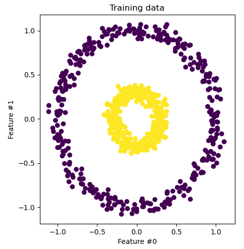
Figure 1: Binary classification dataset that is not linearly separable.
It is easy enough to see that this dataset could not be separated using a hyperplane in 2D. We could separate the two using some nonlinear decision boundary like a circle. If we could transform this into 3D space, we could come up with some features such that it is linearly separable in 3D. For example, let \(\phi(\mathbf{x}) = (x_1^2, x_2^2, \sqrt{2}x_1x_2)\).
Transforming all points and visualizing yields the figure below.
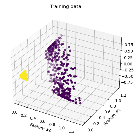
Figure 2: Binary classification dataset transformed into a 3D feature space.
From this perspective, we can clearly see that the data is linearly separable. The question remains: if we only have the original 2D features, how do we compare points in this 3D features space without explicitly transforming each point? The kernel function corresponding to the feature transform above is
\begin{align*} k(\mathbf{x}, \mathbf{x}’) &= (\mathbf{x}^T\mathbf{x}’)^2\\ &= (x_1x’_1 + x_2x’_2)^2\\ &= 2x_1x’_1x_2x’_2 + (x_1x’_1)^2 + (x_2x’_2)^2\\ &= \phi(\mathbf{x})^T \phi(\mathbf{x}’) \end{align*}
where
\[ \phi(\mathbf{x}) = \begin{bmatrix} \sqrt{2}x_1x_2\\ x_1^2\\ x_2^2 \end{bmatrix}. \]
Radial Basis Function Kernel
This kernel follows a Gaussian term and is commonly used with SVMs. It is defined as
\[ k(\mathbf{x}, \mathbf{x’}) = \exp\Big(-\frac{\|\mathbf{x}-\mathbf{x’}\|^2}{2\sigma^2}\Big). \]
Cosine Similarity
Consider the problem of comparing text sequences for a document classification task. One approach is to compare the number of occurrences of each word. The idea is that documents that are similar will have a similar number of words that occur.
\[ k(\mathbf{x}, \mathbf{x}’) = \frac{\mathbf{x}^T \mathbf{x}’}{\|\mathbf{x}\|_2 \|\mathbf{x}’\|_2} \]
Documents that are orthogonal, in the sense that the resulting cosine similarity is 0, are dissimilar. The similarity increases as the score approaches 1. There are several issues with this approach which are addressed by using the term frequence-inverse document frequency (TF-IDF) score.
Constructing Kernels
A valid kernel function must satisfy the following conditions:
- Symmetry: \(k(\mathbf{x}, \mathbf{x}’) = k(\mathbf{x}’, \mathbf{x})\)
- Positive semi-definite: \(k(\mathbf{x}, \mathbf{x}’) \geq 0\)
If the feature space can be represented as a dot product, then it will satisfy the first condition by definition. The second condition can be shown by constructing a Gram matrix \(\mathbf{K}\) and showing that it is positive semi-definite. A matrix \(\mathbf{K}\) is positive semi-definite if and only if \(\mathbf{v}^T\mathbf{K}\mathbf{v} \geq 0\) for all \(\mathbf{v} \in \mathbb{R}^n\).
Direct Construction of a Kernel
In this approach, we define a feature space \(\phi(\mathbf{x})\) and then compute the kernel function as
\[ k(\mathbf{x}, \mathbf{x}’) = \phi(\mathbf{x})^T \phi(\mathbf{x}’). \]
This is the approach used in the example from above. In that example, we used the kernel function \(k(\mathbf{x}, \mathbf{x}’) = (\mathbf{x}^T\mathbf{x}’)^2\). For our 2D input, the feature space is \(\phi(\mathbf{x}) = (x_1^2, x_2^2, \sqrt{2}x_1x_2)\). It is easy to see that the kernel function is the dot product of the feature space, and its kernel matrix is positive semi-definite.
Construction from other valid kernels
As a more convenient approach, it is possible to construct complex kernels from known kernels. Given valid kernels \(k_1(\mathbf{x}, \mathbf{x}’)\) and \(k_2(\mathbf{x}, \mathbf{x}’)\), we can construct a new kernel \(k(\mathbf{x}, \mathbf{x}’)\) using the following operations:
- \(k(\mathbf{x}, \mathbf{x}’) = ck_1(\mathbf{x}, \mathbf{x}’)\) for \(c > 0\)
- \(k(\mathbf{x}, \mathbf{x}’) = f(\mathbf{x})k_1(\mathbf{x}, \mathbf{x}’)f(\mathbf{x}’)\) for \(f(\mathbf{x})\)
- \(k(\mathbf{x}, \mathbf{x}’) = k_1(\mathbf{x}, \mathbf{x}’) + k_2(\mathbf{x}, \mathbf{x}’)\)
- \(k(\mathbf{x}, \mathbf{x}’) = k_1(\mathbf{x}, \mathbf{x}’)k_2(\mathbf{x}, \mathbf{x}’)\)
- \(k(\mathbf{x}, \mathbf{x}’) = \exp(k_1(\mathbf{x}, \mathbf{x}’))\)
- \(k(\mathbf{x}, \mathbf{x}’) = \tanh(k_1(\mathbf{x}, \mathbf{x}’))\)
RBF maps to infinite-dimensional space
It can be shown that the RBF kernel maps the input to an infinite-dimensional space. This is a result of the Taylor series expansion of the exponential function. The RBF kernel is defined as
\[ k(\mathbf{x}, \mathbf{x}’) = \exp\Big(-\frac{\|\mathbf{x}-\mathbf{x’}\|^2}{2\sigma^2}\Big). \]
The Taylor series expansion of the exponential function is
\[ \exp(x) = \sum_{n=0}^\infty \frac{x^n}{n!}. \]
Substituting the RBF kernel into the Taylor series expansion yields
\[ \exp\Big(-\frac{\|\mathbf{x}-\mathbf{x’}\|^2}{2\sigma^2}\Big) = \sum_{n=0}^\infty \frac{\Big(-\frac{\|\mathbf{x}-\mathbf{x’}\|^2}{2\sigma^2}\Big)^n}{n!}. \]
This expansion can be viewed as an infinite sum of polynomial terms. A more formal proof of this result can be found here.
The benefit of this result is that it allows us to work in a high-dimensional space without explicitly transforming the input. This is especially useful when the input space is infinite-dimensional, such as with text data. It is also used to compare the similarity of documents without explicitly transforming the input into a high-dimensional space.