Linear Discriminant Analysis
Slides for these notes can be found here.
Introduction
This section covers classification from a probabilistic perspective. The discriminative approach involves a parameterized function which assigns each input vector \(\mathbf{x}\) to a specific class. We will see that modeling the conditional probability distribution \(p(C_k|\mathbf{x})\) grants us additional benefits while still fulfilling our original classification task.
Let’s begin with a 2 class problem. To classify this with a generative model, we use the class-conditional densities \(p(\mathbf{x}|C_i)\) and class priors \(p(C_i)\). The posterior probability for \(C_1\) can be written in the form of a sigmoid function:
\begin{align*} p(C_1|\mathbf{x}) &= \frac{p(\mathbf{x}|C_1)p(C_1)}{p(\mathbf{x}|C_1)p(C_1) + p(\mathbf{x}|C_2)p(C_2)} \end{align*}
Then multiply the numerator and denominator by
\begin{equation*} \frac{(p(\mathbf{x}|C_1))^{-1}}{(p(\mathbf{x}|C_1))^{-1}}, \end{equation*}
which yields
\begin{equation*} \frac{1}{1 + \frac{p(\mathbf{x}|C_2)p(C_2)}{p(\mathbf{x}|C_1)p(C_1)}}. \end{equation*}
Noting that \(a = \exp(\ln(a))\), we can rewrite further
\begin{equation*} \frac{1}{1 + \exp(-a)}, \end{equation*}
where \(a = \ln \frac{p(\mathbf{x}|C_1)p(C_1)}{p(\mathbf{x}|C_2)p(C_2)}\).
Writing this distribution in the form of the sigmoid function is convenient as it is a natural choice for many other classification models. It also has a very simple derivative which is convenient for models optimized using gradient descent.
Given certain choices for the class conditional densities, the posterior probabilty distribution will be a linear function of the input features:
\begin{equation*} \ln p(C_k|\mathbf{x};\theta) = \mathbf{w}^T \mathbf{x} + c, \end{equation*}
where \(\mathbf{w}\) is a parameter vector based on the parameters of the chosen probability distribution, and \(c\) is a constant term that is not dependent on the parameters. As we will see, the resulting model will take an equivalent form to the discriminative approach.
Gaussian Class Conditional Densities
Let’s assume that our class conditional densities \(p(\mathbf{x}|C_k)\) are Gaussian. We will additionally assume that the covariance matrices between classes are shared. This will result in linear decision boundaries. Since the conditional densities are chosen to be Gaussian, the posterior is given by
\begin{equation*} p(C_k|\mathbf{x};\theta) \propto \pi_k\mathcal{N}(\mathbf{x}|\mathbf{\mu}_c,\Sigma), \end{equation*}
where \(\pi_k\) is the prior probability of class \(k\). We choose to ignore the normalizing constant since it is not dependent on the class.
The class conditional density function for class \(k\) is given by
\begin{equation*} p(\mathbf{x}|C_k;\theta) = \frac{1}{2\pi^{D/2}}\frac{1}{|\Sigma|^{1/2}}\exp\Big(-\frac{1}{2}(\mathbf{x} - \mathbf{\mu}_k)^T \Sigma^{-1} (\mathbf{x} - \mathbf{\mu}_k)\Big). \end{equation*}
Now that we have a concrete function to work with, let’s go back to the simple case of two classes and define \(a = \ln \frac{p(\mathbf{x}|C_1)p(C_1)}{p(\mathbf{x}|C_2)p(C_2)}\). First, we rewrite \(a\):
\begin{equation*} a = \ln p(\mathbf{x}|C_1) - \ln p(\mathbf{x}|C_2) + \ln \frac{p(C_1)}{p(C_2)}. \end{equation*}
The log of the class conditional density for a Gaussian is
\begin{equation*} \ln p(\mathbf{x}|C_k;\mathbf{\mu}_k,\Sigma) = -\frac{D}{2}\ln(2\pi) - \frac{1}{2}\ln|\Sigma|-\frac{1}{2}(\mathbf{x}-\mathbf{\mu}_k)^T \Sigma^{-1} (\mathbf{x}-\mathbf{\mu}_k). \end{equation*}
To simplify the above result, we will group the terms that are not dependent on the class parameters since they are consant:
\begin{equation*} \ln p(\mathbf{x}|C_k;\mathbf{\mu}_k,\Sigma) = -\frac{1}{2}(\mathbf{x}-\mathbf{\mu}_k)^T \Sigma^{-1} (\mathbf{x}-\mathbf{\mu}_k) + c. \end{equation*}
Observing that this quantity takes on a quadratic form, we can rewrite the above as
\begin{equation*} \ln p(\mathbf{x}|C_k;\mathbf{\mu}_k,\Sigma) = -\frac{1}{2}\mathbf{\mu}_k\Sigma^{-1}\mathbf{\mu}_k + \mathbf{x}^T \Sigma^{-1} \mathbf{\mu}_k -\frac{1}{2}\mathbf{x}^T \Sigma^{-1}\mathbf{x} + c. \end{equation*}
Using this, we complete the definition of \(a\):
\begin{align*} a &= \ln p(\mathbf{x}|C_1) - \ln p(\mathbf{x}|C_2) + \ln \frac{p(C_1)}{p(C_2)}\\ &= -\frac{1}{2}\mathbf{\mu}_1\Sigma^{-1}\mathbf{\mu}_1 + \mathbf{x}^T \Sigma^{-1} \mathbf{\mu}_1 + \frac{1}{2}\mathbf{\mu}_2\Sigma^{-1}\mathbf{\mu}_2 - \mathbf{x}^T \Sigma^{-1} \mathbf{\mu}_2 + \ln \frac{p(C_1)}{p(C_2)}\\ &= \mathbf{x}^T(\Sigma^{-1}(\mathbf{\mu}_1 - \mathbf{\mu}_2)) - \frac{1}{2}\mathbf{\mu}_1\Sigma^{-1}\mathbf{\mu}_1 + \frac{1}{2}\mathbf{\mu}_2\Sigma^{-1}\mathbf{\mu}_2 + \ln \frac{p(C_1)}{p(C_2)}\\ &= (\Sigma^{-1}(\mathbf{\mu}_1 - \mathbf{\mu}_2))^T \mathbf{x} - \frac{1}{2}\mathbf{\mu}_1\Sigma^{-1}\mathbf{\mu}_1 + \frac{1}{2}\mathbf{\mu}_2\Sigma^{-1}\mathbf{\mu}_2 + \ln \frac{p(C_1)}{p(C_2)}. \end{align*}
Finally, we define
\begin{equation*} \mathbf{w} = \Sigma^{-1}(\mathbf{\mu}_1 - \mathbf{\mu}_2) \end{equation*}
and
\begin{equation*} w_0 = - \frac{1}{2}\mathbf{\mu}_1\Sigma^{-1}\mathbf{\mu}_1 - \frac{1}{2}\mathbf{\mu}_2\Sigma^{-1}\mathbf{\mu}_2 + \ln \frac{p(C_1)}{p(C_2)}. \end{equation*}
Thus, our posterior takes on the form
\begin{equation*} p(C_1|\mathbf{x};\theta) = \sigma(\mathbf{w}^T \mathbf{x} + w_0). \end{equation*}
Multiple Classes
What if we have more than 2 classes? Recall that a generative classifier is modeled as
\[ p(C_k|\mathbf{x};\mathbf{\theta}) = \frac{p(C_k|\mathbf{\theta})p(\mathbf{x}|C_k, \mathbf{\theta})}{\sum_{k’}p(C_{k’}|\mathbf{\theta})p(\mathbf{x}|C_{k’}, \mathbf{\theta})}. \]
As stated above, \(\mathbf{\pi}_k = p(C_k|\mathbf{\theta})\) and \(p(\mathbf{x}|C_k,\mathbf{\theta}) = \mathcal{N}(\mathbf{x}|\mathbf{\mu}_c,\Sigma)\).
For LDA, the covariance matrices are shared across all classes. This permits a simplification of the class posterior distribution \(p(C_k|\mathbf{x};\mathbf{\theta})\):
\begin{align*} p(C_k|\mathbf{x};\mathbf{\theta}) &\propto \mathbf{\pi}_k \exp\big(\mathbf{\mu}_k^T \mathbf{\Sigma}^{-1}\mathbf{x} - \frac{1}{2}\mathbf{x}^T\mathbf{\Sigma}^{-1}\mathbf{x} - \frac{1}{2}\mathbf{\mu}_k\mathbf{\Sigma}^{-1}\mathbf{\mu}_k\big)\\ &= \exp\big(\mathbf{\mu}_k^T \mathbf{\Sigma}^{-1}\mathbf{x} - \frac{1}{2}\mathbf{\mu}_k\mathbf{\Sigma}^{-1}\mathbf{\mu}_k + \log \mathbf{\pi}_k \big) \exp\big(- \frac{1}{2}\mathbf{x}^T\mathbf{\Sigma}^{-1}\mathbf{x}\big). \end{align*}
The term \(\exp\big(- \frac{1}{2}\mathbf{x}^T\mathbf{\Sigma}^{-1}\mathbf{x}\big)\) is placed aside since it is not dependent on the class \(k\). When divided by the sum per the definition of \(p(C_k|\mathbf{x};\mathbf{\theta})\), it will equal to 1.
Under this formulation, we let
\begin{align*} \mathbf{w}_k &= \mathbf{\Sigma}^{-1}\mathbf{\mu}_k\\ \mathbf{b}_k &= -\frac{1}{2}\mathbf{\mu}_k^T \mathbf{\Sigma}^{-1}\mathbf{\mu}_k + \log \mathbf{\pi}_k. \end{align*}
This lets us express \(p(C_k|\mathbf{x};\mathbf{\theta})\) as the softmax function:
\(p(C_k|\mathbf{x};\mathbf{\theta}) = \frac{\exp(\mathbf{w}_k^T\mathbf{x}+\mathbf{b}_k)}{\sum_{k’}\exp(\mathbf{w}_{k’}^T\mathbf{x}+\mathbf{b}_{k’})}\).
Decision Boundaries
When using LDA, classifications can be made by choosing the class with the highest posterior probability. Geometrically, this decision boundary has a direct connection to logistic regression. The decision boundary is the set of points where the posterior probability of two classes is equal. This is the set of points where the linear discriminant function is equal to 0. This connection follows the derivation given by Kevin P. Murphy in his book Probabilistic Machine Learning: An Introduction (Murphy 2022).
In the previous section, the derivation for the posterior probability of class \(C_k\) was written in the form of the softmax function
\[ p(C_k|\mathbf{x};\mathbf{\theta}) = \frac{\exp(\mathbf{w}_k^T\mathbf{x}+\mathbf{b}_k)}{\sum_{k’}\exp(\mathbf{w}_{k’}^T\mathbf{x}+\mathbf{b}_{k’})}. \]
In the binary case, the posterior for class 1 is given by
\begin{align*} p(C_1|\mathbf{x};\mathbf{\theta}) &= \frac{\exp(\mathbf{w}_1^T\mathbf{x}+\mathbf{b}_1)}{\exp(\mathbf{w}_1^T\mathbf{x}+\mathbf{b}_1) + \exp(\mathbf{w}_2^T\mathbf{x}+\mathbf{b}_2)}\\ &= \frac{1}{1 + \exp((\mathbf{w}_1 - \mathbf{w}_2)^T\mathbf{x}+(\mathbf{b}_1 - \mathbf{b}_2))}\\ &= \sigma((\mathbf{w}_1 - \mathbf{w}_2)^T\mathbf{x}+(\mathbf{b}_1 - \mathbf{b}_2)). \end{align*}
Using the previous definition of \(\mathbf{b}_k\), we can rewrite \(\mathbf{b}_1 - \mathbf{b}_2\) as
\begin{align*} \mathbf{b}_1 - \mathbf{b}_2 &= -\frac{1}{2}\mathbf{\mu}_1^T \mathbf{\Sigma}^{-1}\mathbf{\mu}_1 + \log \mathbf{\pi}_1 + \frac{1}{2}\mathbf{\mu}_2^T \mathbf{\Sigma}^{-1}\mathbf{\mu}_2 - \log \mathbf{\pi}_2\\ &= -\frac{1}{2}(\mathbf{\mu}_1 - \mathbf{\mu}_2)^T \mathbf{\Sigma}^{-1} (\mathbf{\mu}_1 + \mathbf{\mu}_2) + \log \frac{\mathbf{\pi}_1}{\mathbf{\pi}_2}\\ \end{align*}
This can be used to define a new weight vector \(\mathbf{w}’\) and a point directly between the two class means \(\mathbf{x}_0\):
\begin{align*} \mathbf{w}’ &= \mathbf{\Sigma}^{-1}(\mathbf{\mu}_1 - \mathbf{\mu}_2)\\ \mathbf{x}_0 &= \frac{1}{2}(\mathbf{\mu}_1 + \mathbf{\mu}_2) - (\mathbf{\mu}_1 - \mathbf{\mu}_2)\frac{\log \frac{\mathbf{\pi}_1}{\mathbf{\pi}_2}}{(\mathbf{\mu}_1 - \mathbf{\mu}_2)^T \mathbf{\Sigma}^{-1} (\mathbf{\mu}_1 - \mathbf{\mu}_2)}. \end{align*}
With these new terms defined, we have that \(\mathbf{w}’^T\mathbf{x}_0 = -(\mathbf{b}_1 - \mathbf{b}_2)\) and the posterior probability for class 1 can be written in the form of binary logistic regression:
\begin{equation*} p(C_1|\mathbf{x};\mathbf{\theta}) = \sigma(\mathbf{w}’^T(\mathbf{x} - \mathbf{x}_0)). \end{equation*}
Decision Boundary Geometry
Understanding the derivation above is not as important as understanding the result. Remember that $\mathbf{w}^T\mathbf{x}$ returns the coefficient of projection of $\mathbf{x}$ onto $\mathbf{w}$. That number is then passed through the logistic sigmoid function, which gives us a number that we can interpret as the probability of $\mathbf{x}$ belonging to class 1.
The middle point between the two class means \(\mathbf{x}_0\) is the point where the posterior probability of class 1 is 0.5. This is the decision boundary between the two classes. That is, if \(\mathbf{w}’^T\mathbf{x} > \mathbf{w}’^T\mathbf{x}_0\), then the posterior probability of class 1 is greater than \(0.5\) and the input vector \(\mathbf{x}\) is classified as class 1.
The split between the class priors controls the location of the decision boundary. If the class priors are equal, then the decision boundary is the point directly between the two class means. If the class priors are not equal, then the decision boundary is shifted towards the class with the higher prior. The figure below visualizes this.
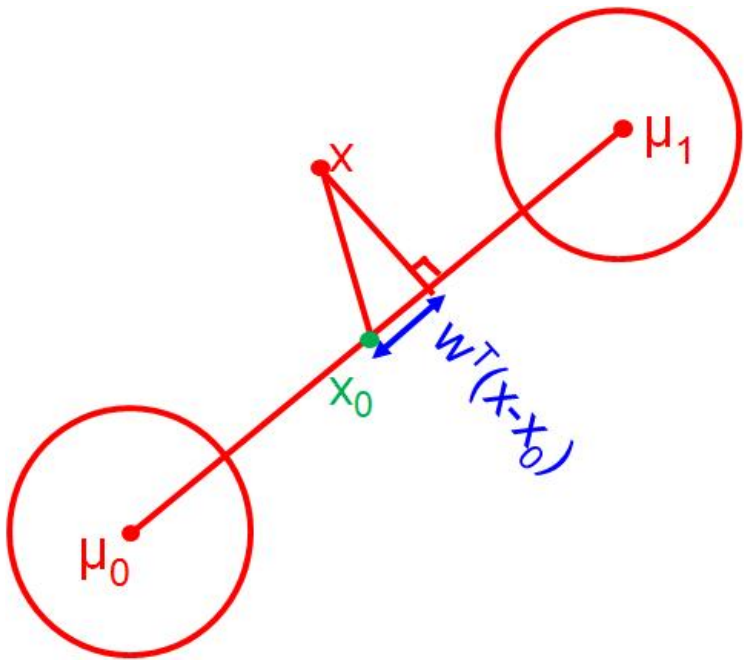
Figure 1: Decision boundary between two classes (Murphy 2022).
Maximum Likelihood Estimation
Given our formulation in the previous section, we can estimate the parameters of the model via maximum likelihood estimation. Assuming \(K\) classes with Gaussian class conditional densities, the likelihood function is
\begin{equation*} p(\mathbf{X}|\mathbf{\theta}) = \prod_{i=1}^n \mathcal{M}(y_i|\mathbf{\pi})\prod_{k=1}^K \mathcal{N}(\mathbf{x}_i|\mathbf{\mu}_k, \mathbf{\Sigma}_k)^{\mathbb{1}(y_i=k)}. \end{equation*}
Taking the log of this function yields
\begin{equation*} \ln p(\mathbf{X}|\mathbf{\theta}) = \Big[\sum_{i=1}^n \sum_{k=1}^K \mathbb{1}(y_i=k)\ln \pi_k\Big] + \sum_{k=1}^K\Big[\sum_{i:y_i=c} \ln \mathcal{N}(\mathbf{x}_n|\mathbf{\mu}_k, \mathbf{\Sigma}_k)\Big]. \end{equation*}
Given that this is a sum of two different components, we can optimize the multinomial parameter \(\mathbf{\pi}\) and the class Gaussian parameters \((\mathbf{\mu}_k, \mathbf{\Sigma}_k)\) separately.
Class Prior
For multinomial distributions, the class prior parameter estimation \(\hat{\pi}_k\) is easily calculated by counting the number of samples belonging to class \(k\) and dividing it by the total number of samples.
\[ \hat{\pi}_k = \frac{n_k}{n} \]
Class Gaussians
The Gaussian parameters can be calculated as discussed during the probability review. The parameter estimates are
\begin{align*} \hat{\mathbf{u}}_k &= \frac{1}{n_k}\sum_{i:y_i=k}\mathbf{x}_i\\ \hat{\Sigma}_k &= \frac{1}{n_k}\sum_{i:y_i=k}(\mathbf{x}_i - \hat{\mathbf{\mu}}_k)(\mathbf{x}_i - \hat{\mathbf{\mu}}_k)^T \end{align*}
The Decision Boundary
The decision boundary between two classes can be visualized at the point when \(p(C_k|\mathbf{x};\theta) = 0.5\).
Quadratic Descriminant Analysis
Linear Discriminant Analysis is a special case of Quadratic Discriminant Analysis (QDA) where the covariance matrices are shared across all classes. Assuming each class conditional density is Gaussian, the posterior probability is given by
\begin{equation*} p(C_k|\mathbf{x};\theta) \propto \pi_k\mathcal{N}(\mathbf{x}|\mathbf{\mu}_k,\Sigma_k). \end{equation*}
Taking the log of this function yields
\begin{equation*} \ln p(C_k|\mathbf{x};\theta) = \ln \pi_k - \frac{1}{2}\ln |\Sigma_k| - \frac{1}{2}(\mathbf{x} - \mathbf{\mu}_k)^T \Sigma_k^{-1}(\mathbf{x} - \mathbf{\mu}_k) + c. \end{equation*}
With LDA, the term \(\frac{1}{2}\ln |\Sigma_k|\) is constant across all classes, so we treat it as another constant. Since QDA considers a different covariance matrix for each class, we must keep this term in the equation.
Quadratic Decision Boundary
In the more general case of QDA, the decision boundary is quadratic, leading to a quadratic discriminant function. As shown above, the posterior probability function for LDA is linear in \(\mathbf{x}\), which leads to a linear discriminant function.
Example
See here for an example using scikit-learn.