Linear Regression
Slides for these notes are available here.
Introduction
Given a dataset of observations \(\mathbf{X} \in \mathbb{R}^{n \times d}\), where \(n\) is the number of samples and \(d\) represents the number of features per sample, and corresponding target values \(\mathbf{Y} \in \mathbb{R}^n\), create a simple prediction model which predicts the target value \(\mathbf{y}\) given a new observation \(\mathbf{x}\). The classic example in this case is a linear model, a function that is a linear combination of the input features and some weights \(\mathbf{w}\).
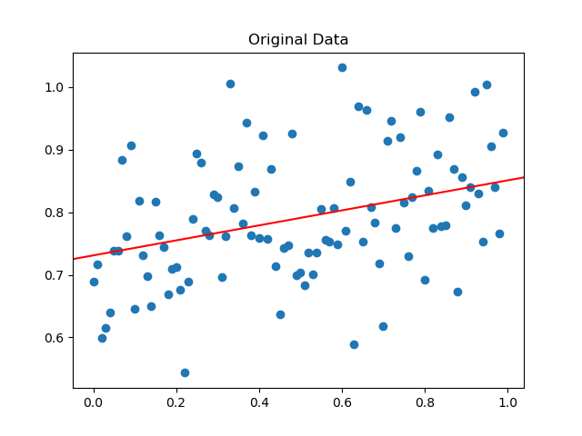
Figure 1: Plot of univariate data where the (x) values are features and (y) are observations.
The generated data is plotted above along with the underlying true function that was used to generate it. If we already know what the true function is, our job is done. Suppose that we only have the data points (in blue). How do we go about modelling it? It is reasonable to first visualize the data and observe that it does follow a linear pattern. Thus, a linear model would be a decent model to choose.
If the data followed a curve, we may decide to fit a polynomial. We will look at an example of that later on. For now, let’s formalize all of the information that we have.
- \((\mathbf{x}, \mathbf{y})\) - Data points from the original dataset. Generally, \(\mathbf{x}\) is a vector of features and \(\mathbf{y}\) is the target vector. In our simple dataset above, these are both scalar values.
- \(\mathbf{w} = (w_0, w_1)\) - Our model parameters. Comparing to the equation \(y = mx + b\), \(w_0\) is our bias term and \(w_1\) is our slope parameter.
Making Predictions
Given \(\mathbf{w}\), we can make a prediction for a new data sample \(\mathbf{x} = x_1\).
\[ h(\mathbf{x}; \mathbf{w}) = w_0 + w_1 x_1 \]
Note that the bias term is always added to the result. We can simplify this into a more general form by appending a constant 1 (s.t. \(x_0 = 1\)) to each of our samples such that \(\mathbf{x} = (1, x_1, …, x_d)\). Then, the general linear model becomes
\[ h(\mathbf{x}; \mathbf{w}) = \sum_{i=0}^{d} w_i x_i = \mathbf{w}^T \mathbf{x}. \]
If our data happened to have more than 1 feature, it would be easy enough to model it appropriately using this notation.
Determining Fitness
If we really wanted to, we could fit our model by plotting it and manually adjusting the weights until our model looked acceptable by some qualitative standard. Fortunately we won’t be doing that. Instead, we will use a quantitative measurement that provides a metric of how well our current parameters fit the data.
For this, we use a cost function or loss function. The most common one to use for this type of model is the least-squares function:
\[ J(\mathbf{w}) = \frac{1}{2}\sum_{i=1}^{n}(h(\mathbf{x}_{i};\mathbf{w}) - \mathbf{y}_{i})^2. \]
Stochastic Gradient Descent
Depending on the random initialization of parameters, our error varies greatly. We can observe that no matter what the chose parameters are, there is no possible way we can achieve an error of 0. The best we can do is minimize this error:
\[ \min_{\mathbf{w}} J(\mathbf{w}). \]
For this, we rely on stochastic gradient descent. The basic idea is as follows:
- Begin with an initial guess for \(\mathbf{w}\).
- Compare the prediction for sample \(\mathbf{x}^{(i)}\) with its target \(\mathbf{y}^{(i)}\).
- Update \(\mathbf{w}\) based on the comparison in part 2.
- Repeat steps 2 and 3 on the dataset until the loss has converged.
Steps 1, 3, and 4 are easy enough. What about step 2? How can we possibly know how to modify \(\mathbf{w}\) such that \(J(\mathbf{w})\) will decrease? By computing the gradient \(\frac{d}{d\mathbf{w}}J(\mathbf{w})\)! How will we know when we have arrived at a minima? When \(\nabla J(\mathbf{w}) = 0\).
\begin{align*} \frac{d}{d\mathbf{w}}J(\mathbf{w}) &= \frac{d}{d\mathbf{w}}\frac{1}{2}(h(\mathbf{x}_{i};\mathbf{w}) - \mathbf{y}_{i})^2\\ &= 2 \cdot \frac{1}{2}(h(\mathbf{x}_{i};\mathbf{w}) - \mathbf{y}_{i}) \cdot \frac{d}{d\mathbf{w}} (h(\mathbf{x}_{i};\mathbf{w}) - \mathbf{y}_{i})\\ &= (h(\mathbf{x}_{i};\mathbf{w}) - \mathbf{y}_{i}) \cdot \frac{d}{d\mathbf{w}} (\mathbf{w}^T \mathbf{x}_{i} - \mathbf{y}_{i})\\ &= (h(\mathbf{x}_{i};\mathbf{w}) - \mathbf{y}_{i}) \mathbf{x}_{i} \end{align*}
The gradient represents the direction of greatest change for a function evaluated With this gradient, we can use an update rule to modify the previous parameter vector \(\mathbf{w}\):
\[ \mathbf{w}_{t+1} = \mathbf{w}_{t} - \alpha \sum_{i=1}^{n} (h(\mathbf{x}_{i};\mathbf{w}_{t}) - \mathbf{y}_{i}) \mathbf{x}_{i}. \]
Here, \(\alpha\) is an update hyperparameter that allows us to control how big or small of a step our weights can take with each update. In general, a smaller value will be more likely to get stuck in local minima. However, too large of a value may never converge to any minima.
Another convenience of this approach is that it is possible to update the weights based on a single sample, batch of samples, or the entire dataset. This sequential process makes optimization using very large dataset feasible.
Probabilistic Interpretation
“Probability theory is nothing but common sense reduced to calculation.” - Pierre-Simon Laplace
Recall Bayes’ theorem:
\[ p(\mathbf{w}|\mathbf{X}) = \frac{p(\mathbf{X}|\mathbf{w})p(\mathbf{w})}{p(\mathbf{X})}. \]
That is, the posterior probability of the weights conditioned on the observered data \(\mathbf{X}\) is equal to the likelihood of the observed data given the times the prior distribution. This base notation doesn’t line up well with our problem. For our problem, we have observations \(\mathbf{Y}\) which are dependent on the input features \(\mathbf{X}\):
\[ p(\mathbf{w}|\mathbf{X}, \mathbf{Y}) = \frac{p(\mathbf{Y}|\mathbf{X}, \mathbf{w}) p(\mathbf{w}|\mathbf{X})}{p(\mathbf{Y}|\mathbf{X})}, \]
where \(\mathbf{X} \in \mathbb{R}^{n \times d}\) and \(\mathbf{Y} \in \mathbb{R}^n\).
The choice of least squares also has statistical motivations. As discussed previously, we are making a reasonable assumption that there is some relationship between the features of the data and the observed output. This is typically modeled assume
\[ \hat{\mathbf{Y}} = f(\mathbf{X}) + \epsilon. \]
Here, \(\epsilon\) is a random error term that is independent of \(\mathbf{X}\) and has 0 mean. This term represents any random noise that occurs either naturally or from sampling. It also includes any effects that are not properly captured by \(f\). Rearranging the terms of this equation to solve for \(\epsilon\) allows us to define the discrepencies in the model:
\[ \mathbf{\epsilon}_i = h(\mathbf{x}_{i}; \mathbf{w}) - \mathbf{y}_{i}. \]
If we assume that these discrepancies are independent and identically distributed with variance \(\sigma^2\) and Gaussian PDF \(f\), the likelihood of observations \(\mathbf{y}^{(i)}\) given parameters \(\mathbf{w}\) is
\[ p(\mathbf{Y}|\mathbf{X}, \mathbf{w}, \sigma) = \prod_{i=1}^{n} f(\epsilon_i; \sigma), \]
where
\[ f(\epsilon_i; \sigma) = \frac{1}{\sqrt{2\pi\sigma^2}}\exp\Big(-\frac{\epsilon^2}{2\sigma^2}\Big). \]
This new parameter changes our original distribution function to
\[ p(\mathbf{w}|\mathbf{X}, \mathbf{Y}, \sigma) = \frac{p(\mathbf{Y}|\mathbf{X}, \mathbf{w}, \sigma) p(\mathbf{w}|\mathbf{X}, \sigma)}{p(\mathbf{Y}|\mathbf{X}, \sigma)}. \]
Two things to note before moving on. First, the prior \(p(\mathbf{Y}|\mathbf{X}, \sigma)\) is a normalizing constant to ensure that the posterior is a valid probability distribution. Second, if we assume that all value for \(\mathbf{w}\) are equally likely, then \(p(\mathbf{w}|\mathbf{x}, \sigma)\) also becomes constant. This is a convenient assumption which implies that maximizing the posterior is equivalent to maximizing the likelihood function.
With that out of the way, we can focus solely on the likelihood function. Expanding out the gaussian PDF \(f\) yields
\[ p(\mathbf{Y}|\mathbf{X}, \mathbf{w}, \sigma) = -\frac{n}{\sqrt{2\pi\sigma^2}}\exp\Big(-\frac{1}{2\sigma^2}\sum_{i=1}^{n}(h(\mathbf{x}_{i};\mathbf{w}) - \mathbf{y}_{i})^2\Big). \]
We can see that maximizing \(p(\mathbf{Y}|\mathbf{X}, \mathbf{w}, \sigma)\) is the same as minimizing the sum of squares. In practice, we use the negative log of the likelihood function since the negative logarithm is monotonically decreasing.
Solving with Normal Equations
You may have studied the normal equations when you took Linear Algebra. The normal equations are motivated by finding approximate solutions to \(A\mathbf{x} = \mathbf{b}\). Most of the earlier part of linear algebra courses focus on finding exact solutions by solving systems of equations using Gaussian elimination (row reduction). Approximate solutions can be found by projecting the observed data points \(\mathbf{b}\) onto the column space of \(A\) and solving \(A \mathbf{x} = \hat{\mathbf{b}}\), where \(\hat{\mathbf{b}} = \text{proj}_{\text{Col} A}\mathbf{b}\). Then, \(\mathbf{b} - \hat{\mathbf{b}}\) represents a vector orthogonal to \(\text{Col}A\).
It is helpful to keep in mind what \(A\), \(\mathbf{x}\), and \(\mathbf{b}\) represent. \(A\) and \(\mathbf{b}\) are the input and output values. If we were trying to predict home prices based on size, each row of \(A\) would represent the size of a different house. In \(\mathbf{b}\) we would record the corresponding prices. We are trying to solve for \(\mathbf{x}\), which is a vector that relates the input to the output.
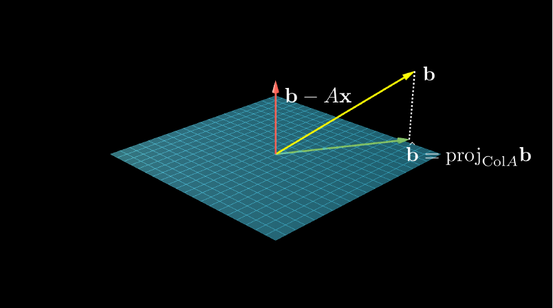
Figure 2: The plane represents every linear combination of the columns of A.
Since each column vector of \(A\) is orthogonal to \(\mathbf{b} - \hat{\mathbf{b}}\), the dot product between them should be 0. Rewriting this, we get
\begin{aligned} A^T(\mathbf{b} - A\mathbf{x}) &= \mathbf{0}\\ A^T \mathbf{b} - A^T A \mathbf{x} &= \mathbf{0}. \end{aligned}
This means that each least-squares solution of \(A\mathbf{x} = \mathbf{b}\) satisfies
\[ A^T A \mathbf{x} = A^T \mathbf{b}. \]
Example
Let’s take our univariate problem of \((\mathbf{x}, \mathbf{y})\) pairs. To use the normal equations to solve the least squares problem, we first change the notation just a bit as not confuse our data points and our parameters:
\[ \mathbf{X}^T \mathbf{X} \beta = \mathbf{X}^T \mathbf{y} \]
Create the design matrix \(\mathbf{X}\) where each row represents the the \(\mathbf{x}\) values. Recall that even though we only have 1 feature for \(\mathbf{x}\), we append the bias constant as \(x_0 = 1\) to account for the bias parameter. \(\mathbf{X}\) is then
\begin{equation*} \mathbf{X} = \begin{bmatrix} x_0^{(0)} & x_1^{(0)}\\ x_0^{(1)} & x_1^{(1)}\\ \vdots & \vdots \\ x_0^{(n)} & x_1^{(n)} \end{bmatrix}. \end{equation*}
The parameter vector is
\begin{equation*} \beta = \begin{bmatrix} \beta_0\\ \beta_1 \end{bmatrix}. \end{equation*}
The observed values are packed into \(\mathbf{y}\). We can then solve for \(\beta\) using any standard solver:
\[ \beta = (\mathbf{X}^T \mathbf{X})^{-1}X^T \mathbf{y}. \]
Rank-Deficient matrices
In the event that the matrix \(\mathbf{X}^T \mathbf{X}\) is singular, then its inverse cannot be computed. This implies that one or more of the features is a linear combination of the others.
This can be detected by checking the rank of \(\mathbf{X}^T \mathbf{X}\) before attempting to compute the inverse. You can also determine which features are redundant via Gaussian elimination. The columns in the reduced matrix that do not have a pivot entry are redundant.
Another Approach to Normal Equations
We can arrive at the normal equations by starting at the probabilistic perspective. Recall the likelihood function
\[ p(\mathbf{Y}|\mathbf{X}, \mathbf{w}, \sigma) = -\frac{n}{\sqrt{2\pi\sigma^2}}\exp\Big(-\frac{1}{2\sigma^2}\sum_{i=1}^{n}(h(\mathbf{x}_{i};\mathbf{w}) - \mathbf{y}_{i})^2\Big). \]
Taking the natural log of this function yields
\[ \ln p(\mathbf{Y}|\mathbf{X}, \mathbf{w}, \sigma) = - \frac{1}{2\sigma^2}\sum_{i=1}^{n}(h(\mathbf{x}_{i}; \mathbf{w}) - \mathbf{y}_{i})^2 - \frac{n}{2}\ln(\sigma^2) - \frac{n}{2}\ln(2\pi). \]
As mentioned before, maximizing the likelihood function is equivalent to minimizing the sum-of-squares function. Thus, we must find the critical point of the likelihood function by computing the gradient (w.r.t. \(\mathbf{w}\)) and solving for 0:
\begin{align*} \nabla \ln p(\mathbf{Y}|\mathbf{X}, \mathbf{w}, \sigma) &= \sum_{i=1}^{n}(\mathbf{w}^T\mathbf{x}_{i} - \mathbf{y}_{i})\mathbf{x}_{i}^{T}\\ &= \mathbf{w}^T \sum_{i=1}^{n}\mathbf{x}_i\mathbf{x}_i^T - \sum_{i=1}^{n}\mathbf{y}_{i}\mathbf{x}_{i}^{T}\\ \end{align*}
Noting that \(\sum_{i=1}^{n}\mathbf{x}_i \mathbf{x}_i^T\) is simply matrix multiplication, we can use
\begin{equation*} \mathbf{X} = \begin{bmatrix} \mathbf{x}_1^T\\ \vdots\\ \mathbf{x}_n^T\\ \end{bmatrix}. \end{equation*}
Then, \(\sum_{i=1}^{n}\mathbf{x}_i \mathbf{x}_i^T = \mathbf{X}^T \mathbf{X}\), \(\sum_{i=1}^{n}\mathbf{y}_i \mathbf{x}_i^T = \mathbf{Y}^T \mathbf{X}\), and
\[ \nabla \ln p(\mathbf{Y}|\mathbf{X}, \mathbf{w}, \sigma) = \mathbf{w}^T \mathbf{X}^T \mathbf{X} - \mathbf{Y}^T \mathbf{X}. \]
Since we are finding the maximum likelihood, we set \(\nabla \ln p(\mathbf{Y}|\mathbf{X}, \mathbf{w}, \sigma) = 0\) and solve for \(\mathbf{w}\):
\[ \mathbf{w} = (\mathbf{X}^T \mathbf{X})^{-1} \mathbf{X}^T \mathbf{Y}. \]
Thus, we arrive again at the normal equations and can solve this using a linear solver.
Fitting Polynomials
Not every dataset can be modeled using a simple line. Data can be exponential or logarithmic in nature. We may also look to use splines to model more complex data.
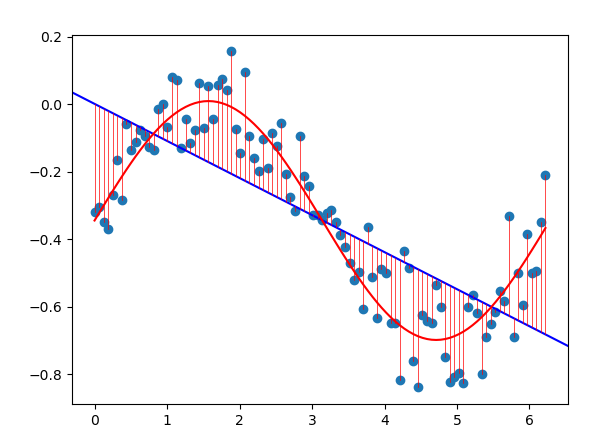
Figure 3: Data generated from a nonlinear function with added noise.
The dataset above was generated from the function as seen in red. Using a simple linear model (blue) does not fit the data well. For cases such as this, we can fit a polynomial to the data by changing our input data.
The simple dataset above has 100 paired samples \((x_i, y_i)\). There is only a single feature \(x_i\) for each sample. It is trivial to determine that the shape of the data follows a cubic function. One solution would be to raise each input to the power of 3. This results in the function (blue) below.
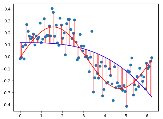
Figure 4: Solution from raising each input to the power of 3.
To fit this data, we need to add more features to our input. Along with the original \(x_i\) features, we will also add \(x_i^2\) and \(x_i^3\). Our data is then 3 dimensional. The figure below shows the least squares fit using the modified data (blue).
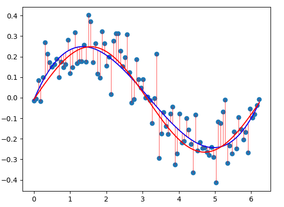
Figure 5: Least squares fit using a polynomial model (blue).
A demo of this can be found here.
Linear Basis Functions
Linear models are linear in their inputs. This formulation is simple, producing models with limited representation. Linear models can be extended as a linear combination of fixed nonlinear functions of the original features. In the previous section, was saw that they could easily be extended to fit polynomial functions.
We now consider creating a model that transforms the original input using one or more nonlinear functions. This type of model is called a linear basis function model.
\[ h(\mathbf{x};\mathbf{w}) = \sum_{j=1}^{m} w_j\phi_j(\mathbf{x}) \]
Common basis functions are the sigmoid, Gaussian, or exponential function. If we choose the \(\sin\) function as a basis function, we can more closely fit our dataset using the least squares approach.
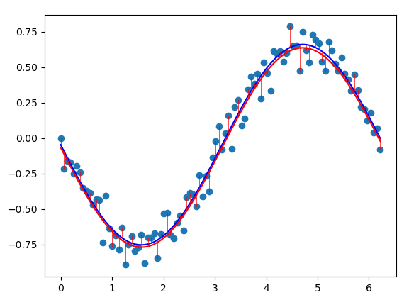
Figure 6: A linear basis function model using the sin function as the choice of basis.