Logistic Regression
Slides for these notes are available here.
Introduction
With Linear Regression we were able to fit a model to our data in order to make inferences on unseen data points. In the examples, both the input features and observation were continuous. With logistic regression, we will use similar models to classify the data points based on their input features. We start out with the simplest approach: we assume that the data is linearly separable and can be assigned one of \(K\) discrete classes.
In the binary case, the target variable will takes on either a 0 or 1. For \(K > 2\), we will use a \(K\) dimensional vector that has a 1 corresponding to the class encoding for that input and a 0 for all other positions. For example, if our possible target classes were \(\{\text{car, truck, person}\}\), then a target vector for \(\text{person}\) would be \(\mathbf{y} = [0, 0, 1]^T\).
This article will stick to a discriminative approach to logistic regression. That is, we define a discriminant function which assigns each data input \(\mathbf{x}\) to a class. For a probabilistic perspective, see Linear Discriminant Analysis.
Picking a Model
We will again start with a linear model \(y = f(\mathbf{x}; \mathbf{w})\). Unlike the model used with Linear Regression, ours will need to predict a discrete class label. The logistic model is often approached by introducing the odds of an event occurring:
\[ \frac{p}{1-p}, \]
where \(p\) is the probability of the event happening. As \(p\) increases, the odds of it happening increase exponentially.
Our input \(p\) represents the probability in range \((0, 1)\) which we want to map to the real number space. To approximate this, we apply the natural logarithm to the odds.
The logistic model assumes a linear relationship between the linear model \(\mathbf{w}^T\mathbf{x}\) and the logit function
\[ \text{logit}(p) = \ln \frac{p}{1-p}. \]
This function maps a value in range \((0, 1)\) to the space of real numbers. Under this assumption, we can write
\[ \text{logit}(p) = \mathbf{w}^T\mathbf{x}. \]
This assumption is reasonable because we ultimately want to predict the probability that an event occurs. The output should then be in the range of \((0, 1)\). If the logit function produces output in the range of real numbers, as does our linear model \(\mathbf{w}^T\mathbf{x}\), then we ultimately want a function that maps from the range of real numbers to to \((0, 1)\).
We can achieve this using the inverse of the logit function, the logistic sigmoid function. It is defined as
\begin{equation*} \sigma(z) = \frac{1}{1 + \exp(-z)}, \end{equation*}
where \(z = \mathbf{w}^T\mathbf{x}\).
The reason for this choice becomes more clear when plotting the function, as seen below.
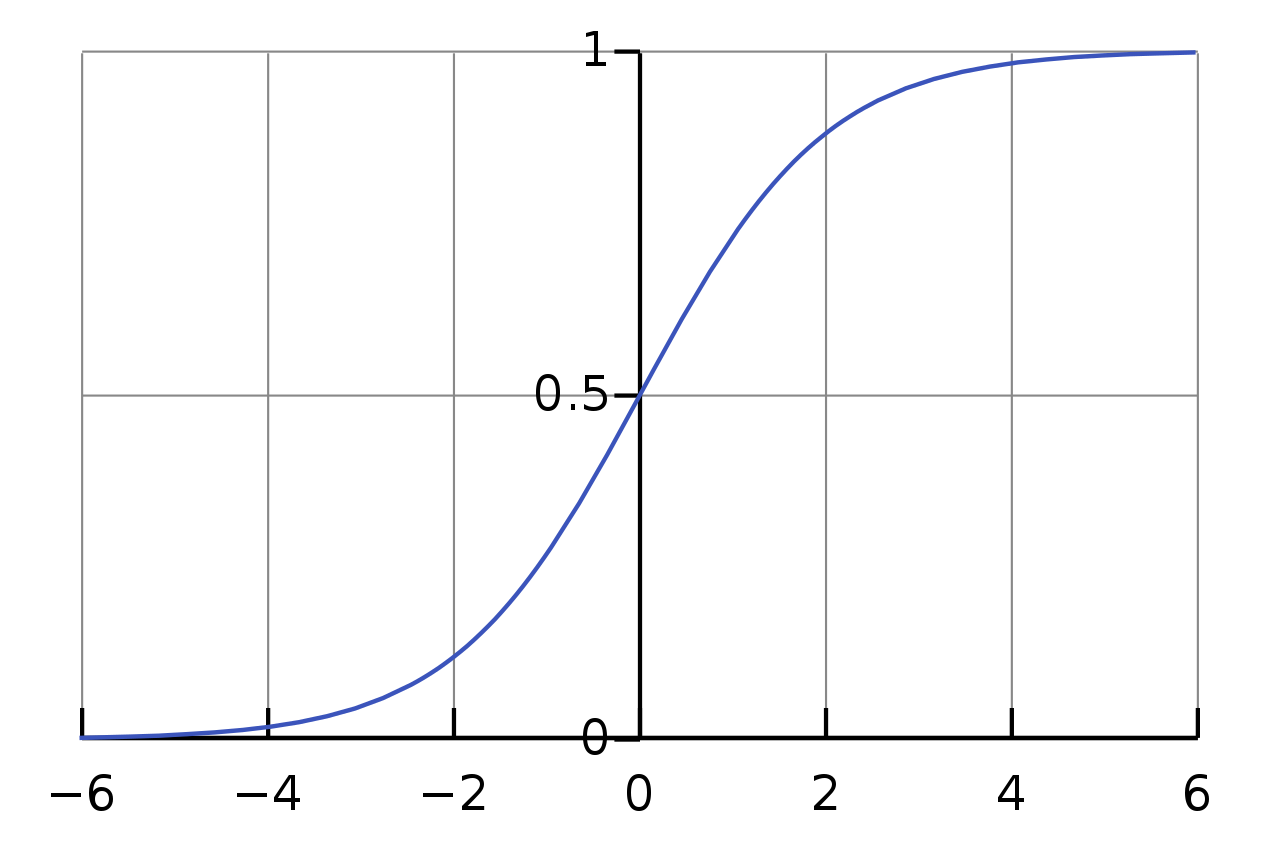
Figure 1: The logistic sigmoid function. Source: Wikipedia
The inputs on the \(x\) axis are clamped to values between 0 and 1. It is also called a squashing function because of this property. This form is also convenient and arises naturally in many probabilistic settings. With this nonlinear activation function, the form of our model becomes
\begin{equation*} f(\mathbf{x};\mathbf{w}) = h(\mathbf{w}^T\mathbf{x}), \end{equation*}
where \(h\) is our choice of activation function.
The logistic sigmoid function also has a convenient derivative, which is useful when solving for the model parameters via gradient descent.
\[ \frac{d}{dx} = \sigma(x)(1 - \sigma(x)) \]
Binary Classification
Consider a simple dataset with 2 features per data sample. Our goal is to classify the data as being one of two possible classes. For now, we’ll drop the activation function so that our model represents a line that separates both groups of data.
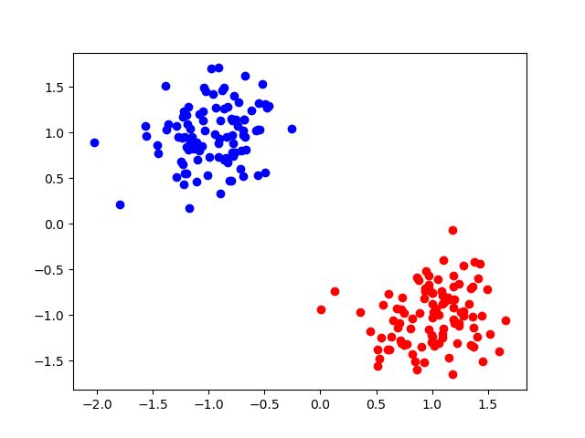
Figure 2: Two groups of data that are very clearly linearly separable.
In the binary case, we are approximating \(p(C_1|\mathbf{x}) = \sigma(\mathbf{w}^T \mathbf{x})\). Then \(p(C_2|\mathbf{x}) = 1 - p(C_1| \mathbf{x})\).
The parameter vector \(\mathbf{w}\) is orthogonal to the decision boundary that separates the two classes. The model output is such that \(f(\mathbf{x};\mathbf{w}) = 0\) when \(\mathbf{x}\) lies on the decision boundary. If \(f(\mathbf{x};\mathbf{w}) \geq 0\) then \(\mathbf{x}\) is assigned to class 1. It is assigned to class 2 otherwise. Since we originally stated that the model should predict either a 0 or 1, we can use the model result as input to the Heaviside step function.
Fitting the Model via Maximum Likelihood
Let \(y_i \in \{0, 1\}\) be the target for binary classification and \(\hat{y}_i \in (0, 1)\) be the output of a logistic regression model. The likelihood function is
\[ p(\mathbf{y}|\mathbf{w}) = \prod_{i=1}^n \hat{y}_i^{y_i}(1 - \hat{y}_i)^{1 - y_i}. \]
Let’s briefly take a look at \(\hat{y}_i^{y_i}(1 - \hat{y}_i)^{1 - y_i}\) to understand the output when the model correctly predicts the \(i^{\text{th}}\) sample or not. Since the output is restricted within the range \((0, 1)\), the model will never produce 0 or 1.
If the target \(y_i = 0\), then we can evaluate the subexpression \(1 - \hat{y}_i\). In this case, the likelihood increases as \(\hat{y}_i\) decreases.
If the target \(y_i = 1\), then we evaluate the subexpression \(\hat{y}_i\).
When fitting this model, we want to define an error measure based on the above function. This is done by taking the negative logarithm of \(p(\mathbf{y}|\mathbf{w})\).
\[ E(\mathbf{w}) = -\ln p(\mathbf{y}|\mathbf{w}) = -\sum_{i=1}^n y_i \ln \hat{y}_i + (1 - y_i) \ln (1 - \hat{y}_i) \]
This function is commonly referred to as the cross-entropy function.
If we use this as an objective function for gradient descent with the understanding that \(\hat{y}_i = \sigma(\mathbf{w}^T \mathbf{x})\), then the gradient of the error function is
\[ \nabla E(\mathbf{w}) = \sum_{i=1}^n (\hat{y}_i - y_i)\mathbf{x}_i. \]
This results in a similar update rule as linear regression, even though the problem itself is different.
Measuring Classifier Performance
How do we determine how well our model is performing?
We will use L1 loss because it works well with discrete outputs. L1 loss is defined as
\begin{equation*} L_1 = \sum_{i}|\hat{y}_i - y_i|, \end{equation*}
where \(\hat{y}_i\) is the ground truth corresponding to \(\mathbf{x}_i\) and \(y_i\) is the output of our model. We can further normalize this loss to bound it between 0 and 1. Either way, a loss of 0 will indicate 100% classification accuracy.
Multiple Classes
In multiclass logistic regression, we are dealing with target values that can take on one of \(k\) values \(y \in \{1, 2, \dots, k\}\). If our goal is to model the distribution over \(K\) classes, a multinomial distribution is the obvious choice. Let \(p(y|\mathbf{x};\theta)\) be a distribution over \(K\) numbers \(w_1, \dots, w_K\) that sum to 1. Our parameterized model cannot be represented exactly by a multinomial distribution, so we will derive it so that it satisfies the same constraints.
We can start by introducing \(K\) parameter vectors \(\mathbf{w}_1, \dots, \mathbf{w}_K \in \mathbb{R}^{d}\), where \(d\) is the number of input features. Then each vector \(\mathbf{w}_k^T \mathbf{x}\) represents \(p(C_k | \mathbf{x};\mathbf{w}_k)\). We need to squash each \(\mathbf{w}_k^T \mathbf{x}\) so that the output sums to 1.
This is accomplished via the softmax function:
\[ p(C_k|\mathbf{x}) = \frac{\exp(\mathbf{w}_k^T \mathbf{x})}{\sum_{j} \exp(\mathbf{w}_j^T \mathbf{x})}. \]
Maximum Likelihood
The target vector for each sample is \(\mathbf{y}_i \in \mathbb{R}^{k}\). Likewise, the output vector \(\hat{\mathbf{y}}_i\) also has \(k\) elements.
The maximum likelihood function for the multiclass setting is given by
\[ p(\mathbf{Y}|\mathbf{W}) = \prod_{i=1}^n \prod_{k=1}^K p(C_k|\mathbf{x}_i)^{y_{ik}} = \prod_{i=1}^n \prod_{k=1}^K \hat{y}_{ik}^{y_{ik}}. \]
\(\mathbf{Y} \in \mathbb{R}^{n \times K}\) is a matrix of all target vectors in the data set. As with the binary case, we can take the negative logarithm of this function to produce an error function.
\[ E(\mathbf{W}) = -\ln p(\mathbf{Y}|\mathbf{W}) = -\sum_{i=1}^n \sum_{k=1}^K y_{ik} \ln \hat{y}_{ik} \]
This is the cross-entropy function for multiclass classification.
The gradient of this function is given as
\[ \nabla_{\mathbf{w}_j}E(\mathbf{W}) = \sum_{i=1}^n (\hat{y}_{ij} - y_{ij}) \mathbf{x}_i. \]
Part of your first assignment will be to work through the derivation of this function. It is standard practice at this point, but it is highly valuable to understand how the result was produced.