Medians and Order Statistics
The lecture slides for these notes are available here.
We briefly touched on a median finding algorithm when discussing Divide and Conquer Algorithms. This section will be a bit of a review, but the point is to touch on the topic of order statistics more generally.
Order Statistics
The \(i^{\text{th}}\) order statistic is the \(i^{\text{th}}\) smallest element in a set of \(n\) elements. The median is the \(\frac{n}{2}^{\text{th}}\) order statistic. The minimum and maximum are the \(1^{\text{st}}\) and \(n^{\text{th}}\) order statistics, respectively. When \(n\) is even, there are two medians:
- the lower median \(\frac{n}{2}^{\text{th}}\) and
- the upper median \(\frac{n}{2} + 1^{\text{th}}\).
The goal of the algorithm of focus in these notes is to determine how select order statistic \(i\) in a set of \(n\) elements. As we saw previously, and will review in these notes, we can use a divide and conquer approach to solve this problem. Further, we will study a linear approach to this problem under the assumption that the elements are distinct.
Minimum and Maximum
One could reason very simply that the lower bound on the number of comparisons needed to find either the minimum or maximum of a set is \(n-1\). One such argument could be that if we left even 1 comparison out of the \(n-1\) comparisons, we could not guarantee that we had found the minimum or maximum. When implementing an algorithm, we would say that an optimal implementation would require \(n-1\) comparisons.
As a quick aside, there are plenty of algorithms that we implement which are not optimal in terms of their theoretical lower bound. Consider a naive matrix multiplication algorithm. There are many redundant reads from memory in this algorithm. For example, if we compute \(C = AB\), we need to calculate the output values \(C_{1, 1}\) and \(C_{1, 2}\), among others. Both of these outputs require reading from the first row of \(A\).
We could find both the minimum and maximum of a set in \(2n - 2\) operations by passing over the set twice. This is theoretically optimal since each pass is performing the optimal \(n-1\) comparisons. If we first compared a pair of elements with each other before comparing them to the minimum and maximum, respectively, we could find both the minimum and maximum in \(3\left\lfloor\frac{n}{2}\right\rfloor\) comparisons.
Selection in expected linear time
We now turn to the problem of selection. Given a set of \(n\) elements and an integer \(i\), we want to find the \(i^{\text{th}}\) order statistic. We will assume that all elements are distinct. We will also assume that \(i\) is between 1 and \(n\).
The randomized select algorithm returns the \(i^{\text{th}}\) smallest element of an array bounded between indices \(p\) and \(r\). It relies on randomized_partition, just like Quicksort.
def randomized_select(A, p, r, i):
    if p == r:
        return A[p]
    q = randomized_partition(A, p, r)
    k = q - p + 1
    if i == k:
        return A[q]
    elif i < k:
        return randomized_select(A, p, q-1, i)
    else:
        return randomized_select(A, q+1, r, i-k)
The first conditional checks if the array had only a single element, in which case it must be the value we are looking for. If not, the array is partitioned so that each element in \(A[p:q-1]\) is less than or equal to \(A[q]\) which is less than or equal to the elements in \(A[q+1:r]\). The line \(k = q - p + 1\) calculates the number of elements less than or equal to the pivot. If the index we are looking for is equal to this number, then we have found it and can return the value immediately.
If the value was not yet found and \(i < k\), then \(i\) must be in the subarray \(A[p:q-1]\). Therefore, the function is recursively called on that subarray. Otherwise, the subarray \(A[q+1:r]\) is checked. An example from Cormen et al. is shown below (Cormen et al. 2022).
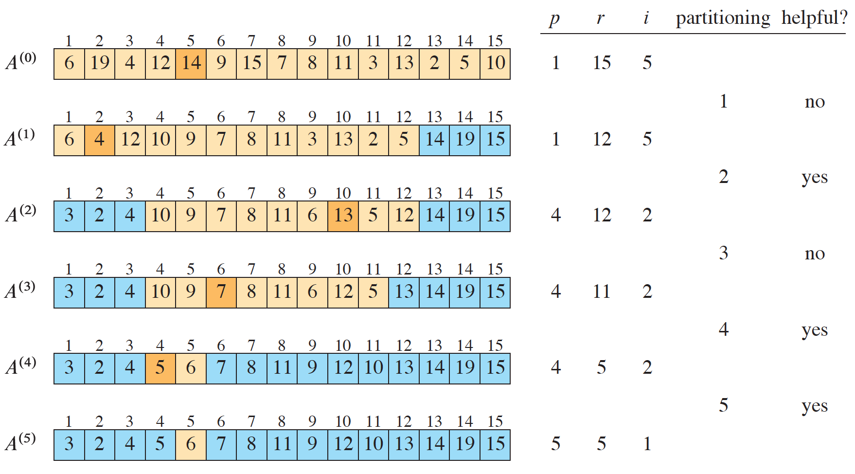
Figure 1: Randomized select from (Cormen et al. 2022).
Explanation of figure \(A^{(0)}\) shows that \(A[5] = 14\) was chosen as the pivot. The next row, \(A^{(1)}\), depicts the completed partitioning. Cormen et al. note that this is not a helpful partitioning since less than \(\frac{1}{4}\) of the elements are ignored. A helpful partition is one that leaves at most \(\frac{3}{4}\) of the elements after the partitioning.
Analysis
The worst-case running time of randomized_select is \(O(n^2)\) since we are partitioning \(n\) elements at \(\Theta(n)\) each. Since the pivot of randomized_partition is selected at random, we can expect a good split at least every 2 times it is called. The proof for this is similar to the one made when analyzing Quicksort. Briefly, the expected number of times we must partition before we get a helpful split is 2, which only doubles the running time. The recurrence is still \(T(n) = T(3n/4) + \Theta(n) = \Theta(n)\).
The first step to showing that the expected runtime of randomized_select is \(\Theta(n)\) is to show that a partitioning is helpful with probability at least \(\frac{1}{2}\) (Cormen et al. 2022). The rest of the proof requires further examination and comprehension.
The proof presented by Cormen et al. begins with the following terms:
- \(h_i\) is the event that the \(i^{\text{th}}\) partitioning is helpful.
- \(\{h_0, h_1, \dots, h_m\}\) is the sequence of helpful partitionings.
- \(n_k = |A^{(h_k)}|\) is the number of elements in the subarray \(A^{(h_k)}\) at the \(k^{\text{th}}\) partitioning.
- \(n_k \leq (3/4)n_{k-1}\) for \(k \geq 1\), or \(n_k \leq (3/4)^kn_0\).
- \(X_k = h_{k+1} - h_k\) is the number of unhelpful partitionings between the \(k^{\text{th}}\) and \((k+1)^{\text{th}}\) helpful partitionings.
There are certainly partitionings that are not helpful. These are depicted as subarrays within each generation of helpful partitionings. The figure below exemplifies this.
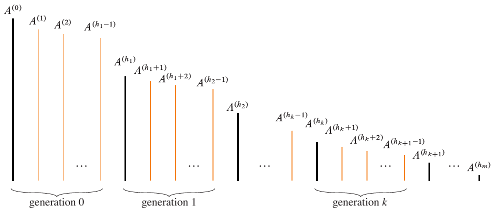
Figure 2: The sets within each generation of helpful partitionings are not helpful. From (Cormen et al. 2022).
Given that the probability that a partitioning is helpful is at least \(\frac{1}{2}\), we know that \(E[X_k] \leq 2\). With this, an upper bound on the number of comparisons of partitioning is derived. The total number of comparisons made when partitioning is less than
\begin{align*} \sum_{k=0}^{m-1} \sum_{j=h_k}^{h_k + X_k - 1} |A^{(j)}| &\leq \sum_{k=0}^{m-1} \sum_{j=h_k}^{h_k + X_k - 1} |A^{(h_k)}| \\ &= \sum_{k=0}^{m-1} X_k|A^{(h_k)}| \\ &\leq \sum_{k=0}^{m-1} X_k \left(\frac{3}{4}\right)^k n_0. \\ \end{align*}
The first term on the first line represents the total number of comparisons across all sets. The first sum loops through the \(m\) helpful partitionings, and the inner loop sums the number of comparisons made for each unhelpful partitioning. It is bounded by the term on the right. This is because \(|A^{(j)}| \leq |A^{(h_k)}|\) if \(A^{(j)}\) is in the \(k^{\text{th}}\) generation of helpful partitionings (see term 4 above).
Using term 5 from above, the second line is derived. The third line leverages term 4 again. The sum is a geometric series, and the total number of comparisons is less than
\begin{align*} \text{E} \left[\sum_{k=0}^{m-1} X_k \left(\frac{3}{4}\right)^k n_0\right] &= n_0 \sum_{k=0}^{m-1} \left(\frac{3}{4}\right)^k \text{E}[X_k]\\ &\leq 2n_0 \sum_{k=0}^{m-1} \left(\frac{3}{4}\right)^k \\ &< 2n_0 \sum_{k=0}^{\infty} \left(\frac{3}{4}\right)^k \\ &= 8n_0. \end{align*}
The last line is the result of a geometric series. This concludes the proof that randomized_partition runs in expected linear time.
Worst-Case Linear Time
Partition-around partitions the input around a specific pivot. I assume this is meant to be the median.
Select Algorithm
Select returns the i-th smallest element. The first loop increments the left border index until the remaining number of elements is divisible by 5. This is so the array can be split into groups of 5 following the same process as the median of medians algorithm. This will also return \(A[p]\) if it happens to coincide with the element the user was looking for.
The proof largely follows the same one laid out for the median of medians algorithm. After all, it is almost identical with the exception that the original algorithm discussed did not necessarily need to preprocess the input to be divisible by 5. This preprocessing step only takes \(O(1)\) time and is thus irrelevant.
Problems and Exercises
- Show that the second largest of \(n\) elements can be found with \(n + \lceil\log_2 n\rceil - 2\) comparisons in the worst case.