Naive Bayes
Slides for these notes can be found here.
Introduction
To motivate naive Bayes classifiers, let’s look at slightly more complex data. The MNIST dataset was one of the standard benchmarks for computer vision classification algorithms for a long time. It remains useful for educational purposes. The dataset consists of 60,000 training images and 10,000 testing images of size \(28 \times 28\). These images depict handwritten digits. For the purposes of this section, we will work with binary version of the images. This implies that each data sample has 784 binary features.
We will use the naive Bayes classifier to make an image classification model which predicts the class of digit given a new image. Each image will be represented by a vector \(\mathbf{x} \in \mathbb{R}^{784}\). Modeling \(p(\mathbf{x}|C_k)\) with a multinomial distribution would require \(10 \times 2^{784} - 10\) parameters since there are 10 classes and 784 features.
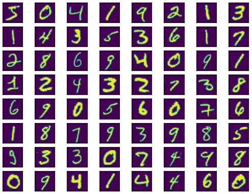
Figure 1: Samples of the MNIST training dataset.
With the naive assumption that the features are independent conditioned on the class, the number model parameters becomes \(10 \times 784\).
Definition
A naive Bayes classifier makes the assumption that the features of the data are independent. That is, \[ p(\mathbf{x}|C_k, \mathbf{\theta}) = \prod_{d=1}^D p(x_i|C_k, \theta_{dk}), \] where \(\mathbf{\theta}_{dk}\) are the parameters for the class conditional density for class \(k\) and feature \(d\). Using the MNIST dataset, \(\mathbf{\theta}_{dk} \in \mathbb{R}^{784}\). The posterior distribution is then
\begin{equation*} p(C_k|\mathbf{x},\mathbf{\theta}) = \frac{p(C_k|\mathbf{\pi})\prod_{i=1}^Dp(x_i|C_k, \mathbf{\theta}_{dk})}{\sum_{k’}p(C_{k’}|\mathbf{\pi})\prod_{i=1}^Dp(x_i|C_{k’},\mathbf{\theta}_{dk’})}. \end{equation*}
If we convert the input images to binary, the class conditional density \(p(\mathbf{x}|C_k, \mathbf{\theta})\) takes on the Bernoulli pdf. That is,
\begin{equation*} p(\mathbf{x}|C_k, \mathbf{\theta}) = \prod_{i=1}^D\text{Ber}(x_i|\mathbf{\theta}_{dk}). \end{equation*}
The parameter \(\theta_{dk}\) is the probability that the feature \(x_i=1\) given class \(C_k\).
Maximum Likelihood Estimation
Fitting a naive Bayes classifier is relatively simple using MLE. The likelihood is given by
\begin{equation*} p(\mathbf{X}, \mathbf{y}|\mathbf{\theta}) = \prod_{n=1}^N \mathcal{M}(y_n|\mathbf{\pi})\prod_{d=1}^D\prod_{k=1}^{K}p(x_{nd}|\mathbf{\theta}_{dk})^{\mathbb{1}(y_n=k)}. \end{equation*}
To derive the estimators, we first take the log of the likelihood:
\begin{equation*} \ln p(\mathbf{X}, \mathbf{y}|\mathbf{\theta}) = \Bigg[\sum_{n=1}^N\sum_{k=1}^K \mathbb{1}(y_n = k)\ln \pi_k\Bigg] + \sum_{k=1}^K\sum_{d=1}^D\Bigg[\sum_{n:y_n=k}\ln p(x_{nd}|\theta_{dk})\Bigg]. \end{equation*}
Thus, we have a term for the the multinomial and terms for the class-feature parameters. As with previous models that use a multinomial form, the parameter estimate for the first term is computed as
\begin{equation*} \hat{\pi}_k = \frac{N_k}{N}. \end{equation*}
The features used in our data are binary, so the parameter estimate for each \(\hat{\theta}_{dk}\) follows the Bernoulli distribution:
\begin{equation*} \hat{\theta}_{dk} = \frac{N_{dk}}{N_{k}}. \end{equation*}
That is, the number of times that feature \(d\) is in an example of class \(k\) divided by the total number of samples for class \(k\).
Making a Decision
Given parameters \(\mathbf{\theta}\), how can we classify a given data sample?
\begin{equation*} \text{arg}\max_{k}p(y=k)\prod_{i}p(x_i|y=k) \end{equation*}
Relation to Multinomial Logistic Regression
Consider some data with discrete features having one of \(K\) states, then \(x_{dk} = \mathbb{1}(x_d=k)\). The class conditional density, in this case, follows a multinomial distribution:
\[ p(\mathbf{x} \vert y = c, \mathbf{\theta}) = \prod_{d=1}^D \prod_{k=1}^K \theta_{dck}^{x_{dk}}. \]
We can see a connection between naive Bayes and logistic regression when we evaluate the posterior over classes:
\begin{align*} p(y=c|\mathbf{x}, \mathbf{\theta}) &= \frac{p(y=c)p(\mathbf{x}|y=c, \mathbf{\theta})}{p(\mathbf{x})}\\ &= \frac{\pi_c \prod_{d} \prod_{k} \theta_{dck}^{x_{dk}}}{\sum_{c’}\pi_{c’}\prod_{d}\prod_{k}\theta_{dc’k}^{x_{dk}}} \\ &= \frac{\exp[\log \pi_c + \sum_d \sum_k x_{dk}\log \theta_{dck}]}{\sum_{c’} \exp[\log \pi_{c’} + \sum_d \sum_k x_{dk} \log \theta_{dc’k}]}. \end{align*}
This has the same form as the softmax function:
\[ p(y=c|\mathbf{x}, \mathbf{\theta}) = \frac{e^{\beta^{T}_c \mathbf{x} + \gamma_c}}{\sum_{c’=1}^C e^{\beta^{T}_{c’}\mathbf{x} + \gamma_{c’}}} \]
MNIST Example
With the model definition and parameter estimates defined, we can fit and evaluate the model. Using scikit-learn, we fit a Bernoulli naive Bayes classifier on the MNIST training set: Naive Bayes.
Gaussian Formulation
If our features are continuous, we would model them with univariate Gaussians.