Probability Theory
Slides for these notes are available here. Additional slides on Gaussian distributions are here.
Introduction
Probability theory provides a consistent framework for the quantification and manipulation of uncertainty. It allows us to make the best decisions given the limited information we may have. Many tasks, models, and evaluation metrics that we will explore in this course are either based on, or are inspired by, probability theory.
A Simple Example
Scenario: There are two cookie jars, a blue one for cookies with oatmeal raisin cookies and a red one for chocolate chip cookies. The jar with oatmeal raisin cookies has 8 cookies in it. The chocolate chip jar has 10 cookies. Some monster took 2 of the chocolate chip cookies and placed them in the oatmeal raisin jar and placed 1 of the oatmeal raisin cookies in the chocolate chip jar. Thus, the oatmeal raisin jar has 2 chocolate chip and 7 oatmeal raisin. The chocolate chip jar has 8 chocolate chip and 1 oatmeal raisin.
Let’s say that we pick the chocolate chip jar 80% of the time and the oatmeal raisin jar 20% of the time. For a given jar, the cookies inside are all equally likely to be picked. We can assign this probability to random variables:
- \(J\) - The type of jar, either blue \(b\) or red \(r\).
- \(C\) - The type of cookie, either oatmeal \(o\) or chocolate chip \(c\).
We can define the probability of picking a particular jar:
- \(p(J=b) = 0.2\)
- \(p(J = r) = 0.8\)
Notice that their sum is 1.0. These probabilities can be estimated empirically given an observer recording the events. We may also define the probabilities of picking a particular type of cookie.
- \(p(C = o)\)
- \(p(C = c)\)
For each jar, the probabilities of picking the cookies must sum to 1. The tables below show the individual probabilities of picking each type of cookie from each jar. Since we can observe the actual quantities, we can define the probabilities empirically.
| Chocolate Chip | Oatmeal Raisin | |
|---|---|---|
| Blue Jar | 2 / 9 = 0.222 | 7 / 9 = 0.778 |
| Chocolate Chip | Oatmeal Raisin | |
|---|---|---|
| Red Jar | 8 / 9 = 0.889 | 1 / 9 = 0.111 |
Given these quantities, we can ask slightly more complicated questions such as “what is the probability that I will select the red jar AND take a chocolate chip cookie?” This is expressed as a joint probability distribution, written as \(p(J = r, C = c)\). It is defined based on two events:
- the prior probability of picking the red jar,
- the conditional probability of picking a chocolate chip cookie conditioned on the event that the red jar was picked.
\begin{equation*} p(J=r, C=c) = p(C=c | J=r) p(J = r) \end{equation*}
This is also referred to as the product rule.
We already know \(p(J=r) = 0.8\). From the table above, we can see that \(p(C=c|J=r) = 0.889\). Thus, \(p(C=c,J=r) = 0.8 * 0.889 = 0.711\).
If we knew nothing about the contents of the jar or the prior probabilities of selecting a jar, we could measure the joint probability empirically. This would simply be the number of times we select the red jar AND a chocolate chip cookie divided by total number of trials. For best results, perform an infinite number of trials.
If instead we wanted to measure the conditional probability \(p(C=c|J=r)\), we would simply take the number of times a chocolate chip cookie is taken from the red jar and divide by the total number of times the red jar was selected.
We can construct a joint probability table given the joint probabilities of all the events listed.
| Chocolate Chip | Oatmeal Raisin | |
|---|---|---|
| Red Jar | 0.711 | 0.089 |
| Blue Jar | 0.044 | 0.156 |
If you summed each row and further took the sum of the sum of rows, you would get 1. Likewise, the sum of the sum of columns would equal 1.
Summing the columns for each row yields the prior probability of selecting each type of jar. Similarly, summing the rows for each column gives the prior probability of selecting that type of cookie. This is referred to as the marginal probability or sum rule, which is computed by summing out the other variables in the joint distribution. For example,
\begin{equation*} p(x_i) = \sum_j p(x_i, y_j) \end{equation*}
Empirically, this is computed as the number of times event \(x_i\) occurs out of ALL trials.
Although the joint probabilities \(p(X, Y)\) and \(p(Y, X)\) would be written slightly differently, they are equal. With this in mind, we can set them equal to each other to derive Bayes’ rule:
\begin{align*} p(X, Y) &= p(Y, X)\\ p(X|Y)p(Y) &= p(Y|X)p(X)\\ p(X|Y) &= \frac{p(Y|X)p(X)}{p(Y)} \end{align*}
In this context, \(p(X|Y)\) is referred to as the posterior probability of event \(X\) conditioned on the fact that we know event \(Y\) has occurred. On the right, \(p(X)\) is the prior probability of event \(X\) in the absence of any additional evidence.
Two variables are independent, then
\[ p(X, Y) = p(X)p(Y) \]
If two variables are conditionally independent given a third event, then
\[ p(X, Y|Z) = P(X|Z)P(Y|Z) \]
Probability Distributions
Events come from a space of possible outcomes.
\begin{equation*} \Omega = {1, 2, 3, 4, 5, 6} \end{equation*}
A measureable event is one for which we can assign a probability.
An event space must satisfy the following:
- It contains the empty event \(\emptyset\) and trivial event \(\Omega\)
- It is closed under union
- It is closed under complementation: if \(\alpha \in S\), so is \(\Omega - \alpha\)
- Statement 2 implies difference and intersection
A probability distribution \(P\) over \((\Omega, S)\) maps events \(S\) to real values and satisfies:
- \(P(\alpha) \geq 0\) for all \(\alpha \in S\)
- \(P(\Omega) = 1\)
- If \(\alpha,\beta \in S\) and \(\alpha \cap \beta = \emptyset\), then \(P(\alpha \cup \beta) = P(\alpha)+P(\beta)\)
- \(P(\emptyset) = 0\)
- \(P(\alpha \cup \beta) = P(\alpha) + P(\beta) - P(\alpha \cap \beta)\)
Conditional Probability
Defined as
\begin{equation*} P(\beta | \alpha) = \frac{P(\alpha \cap \beta)}{P(\alpha)} \end{equation*}
The more that \(\alpha\) and \(\beta\) relate, the higher the probability.
The Chain Rule of Probability
\begin{equation*} P(\alpha \cap \beta) = P(\alpha) P(\beta | \alpha) \end{equation*}
Generally…
\begin{equation*} P(\alpha_1 \cap \dotsb \cap \alpha_k) = P(\alpha_1)P(\alpha_2 | \alpha_1) \dotsm P(\alpha_k | \alpha_1 \cap \dotsb \cap \alpha_{k-1}) \end{equation*}
Bayes’ Rule
\begin{equation*} P(\alpha | \beta) = \frac{P(\beta | \alpha)P(\alpha)}{P(\beta)} \end{equation*}
Computes the inverse conditional probability.
A general conditional version of Baye’s rule:
\begin{equation*} P(\alpha | \beta \cap \gamma) = \frac{P(\beta | \alpha \cap \gamma)P(\alpha | \gamma)}{P(\beta | \gamma)} \end{equation*}
Example: TB Tests A common example for introduction Bayes’ rule is that of the test that gives 95% accuracy. The naive assumption here is that if you receive a positive result with no prior information, then there is a 95% chance you have the infection. This is wrong because that value is conditioned on already being infected.
Rules of Probability
Sum Rule: \(p(X) = \sum_{Y}p(X, Y)\)
Product Rule: \(p(X, Y) = p(Y|X)p(X)\)
Random Variables
Allows for compact notation when talking about an event. It can also be represented as a function:
\begin{equation*} f_{\text{Grade}} \end{equation*}
maps each person in \(\Omega\) to a grade value.
Random variables are commonly either categorical or real numbers.
The multinoulli distribution is one over \(k > 2\) categorical random variables. If \(k = 2\), the distribution is called the Bernoulli or binomial distribution.
The marginal distribution is one over a single random variable \(X\).
A joint distribution is one over a set of random variables.
The marginal can be computed from a joint distribution.
\begin{equation*} P(x) = \sum_{y}P(x, y) \end{equation*}
Continuous Variables
The introductory example looked at events that take on discrete values. That is, we either selected a cookie or did not. Most of the problems we will deal with in this course involve continuous values. In this case, we are concerned with intervals that the values may take on. If we consider a small differential of our random variable \(x\) as \(\delta x\), we can compute the probability density \(p(x)\).
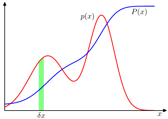
Figure 1: PDF (p(x)) and CDF (P(x)). Source: Bishop
With this differential \(\delta x\), we can compute the probability that \(x\) lies on some interval \((a, b)\):
\begin{equation*} p(a \leq x \leq b) = \int_{a}^{b} p(x) dx \end{equation*}
As with discrete probability distributions, the probability density must sum to 1 and cannot take a negative value. That is
\begin{align*} p(x) &\geq 0\\ \int_{-\infty}^{\infty}p(x)dx &= 1 \end{align*}
In the plot above, \(p(x)\) is the probability density function (pdf) and \(P(x)\) is the cumulative distribution function (cdf). It is possible for a pdf to have a value greater than 1, as long as integrals over any interval are less than or equal to 1.
The cumulative distribution function \(P(x)\) is the probability that \(x\) lies in the interval \((-\infty, z)\), given by
\begin{equation*} P(z) = \int_{\infty}^{z} p(x)dx. \end{equation*}
Note that the derivative of the cdf is equal to the pdf.
The product rule for continuous probability distributions takes on the same form as that of discrete distributions. The sum rule is written in terms of integration:
\begin{equation*} p(x) = \int p(x, y)dy. \end{equation*}
Moments of a Distribution
A moment of a function describes a quantitative measurement related to its graph. With respect to probability densities, the $k$th moment of \(p(x)\) is defined as \(\mathbb{E}[x^k]\). The first moment is the mean of the distribution, the second moment is the variance, and the third moment is the skewness.
Three extremely important statistics for any probability distribution are the average, variance, and covariance.
Expectation
The average of a function \(f(x)\) under a probability distribution \(p(x)\) is referred to as the expectation of \(f(x)\), written as \(\mathbb{E}[f]\). The expectation for discrete and continuous distributions are
\begin{align*} \mathbb{E}[f] &= \sum_x p(x)f(x) \text{ and}\\ \mathbb{E}[f] &= \int p(x)f(x)dx, \end{align*}
respectively.
](/ox-hugo/2022-01-25_17-56-37_screenshot.png)
Figure 2: Expectation of rolling a d6 over ~1800 trials converges to 3.5. Source: Seeing Theory
The mean value for a discrete and continuous probability distribution is define as
\begin{align*} \mathbb{E}[f] &= \sum_x p(x)x \text{ and}\\ \mathbb{E}[f] &= \int_{-\infty}^{\infty} p(x)xdx, \end{align*}
respectively.
Empirically, we can approximate this quantity given \(N\) samples as
\begin{equation*} \mathbb{E}[f] \approx \frac{1}{N}\sum_{i=1}^{N}f(x_i). \end{equation*}
Variance
The variance of a function \(f(x)\) under a probability distribution \(p(x)\) measures how much variability is in \(f(x)\) around the expected value \(\mathbb{E}[f(x)]\) and is defined by
\begin{align*} \text{var}[f] &= \mathbb{E}[(f(x) - \mathbb{E}[f(x)])^2]\\ &= \mathbb{E}[f(x)^2] - \mathbb{E}[f(x)]^2. \end{align*}
](/ox-hugo/2022-01-25_18-02-03_screenshot.png)
Figure 3: Variance of drawing cars with values 1-10 100 trials converges to 8.79. True variance is 8.25. Source: Seeing Theory
Covariance
The covariance of two random variables \(x\) and \(y\) provides a measure of dependence between the two variables. This implies that the covariance between two independent variables is 0.
\begin{align*} \text{cov}[\mathbf{x},\mathbf{y}] &= \mathbf{E}_{\mathbf{x},\mathbf{y}}[\{\mathbf{x} - \mathbb{E}[\mathbf{x}]\}\{\mathbf{y}^T - \mathbb{E}[\mathbf{y}^T]\}]\\ &= \mathbb{E}_{\mathbf{x},\mathbf{y}}[\mathbf{x}\mathbf{y}^T] - \mathbb{E}[\mathbf{x}]\mathbb{E}[\mathbf{y}^T]. \end{align*}
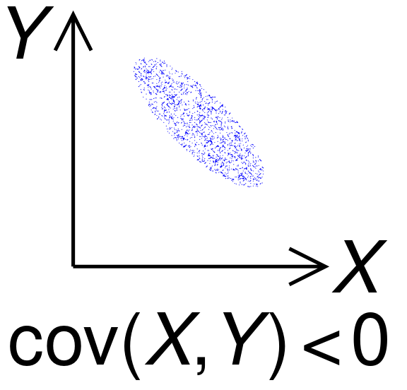
Figure 4: Plot of 2D data with negative covariance. Source: Wikipedia
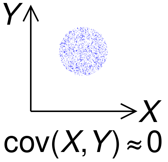
Figure 5: Plot of 2D data with approximately 0 covariance. Source: Wikipedia
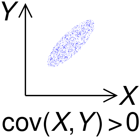
Figure 6: Plot of data with positive covariance. Source: Wikipedia
Correlation
The correlation between two random variables \(x\) and \(y\) relates to their covariance, but it is normalized to lie between -1 and 1.
\begin{equation*} \text{corr}[\mathbf{x},\mathbf{y}] = \frac{\text{cov}[\mathbf{x},\mathbf{y}]}{\sqrt{\text{var}[\mathbf{x}]\text{var}[\mathbf{y}]}} \end{equation*}
The correlation between two variables will equal 1 if there is a linear relationship between them. We can then view the correlation as providing a measurement of linearity.
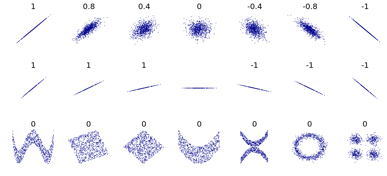
Figure 7: Sets of points with their correlation coefficients. Source: Wikipedia
Limitations of Moments
Summary statistics can be useful but do not tell the whole story of your data. When possible, it is always better to visualize the data. An example of this is the Anscombosaurus, derived from the Anscombe’s quartet. The quartet consists of four datasets that have nearly identical summary statistics but are visually distinct. A modern version, called the Datasaurus Dozen, consists of 12 datasets that have the same summary statistics but are visually distinct.
)](/ox-hugo/2023-08-29_21-15-04_screenshot.png)
Figure 8: Datasaurus Dozen (source: Same Stats, Different Graphs: Generating Datasets with Varied Appearance and Identical Statistics through Simulated Annealing)