Regularization
Slides for these notes are available here.
Introduction
Regularization is any modification we make to a learning algorithm that is intended to reduce its generalization error but not its training error. - Goodfellow et al.
Regularization comes in many forms. Some techniques may add an additional penalty to the loss function. Others, such as data augmentation, add artificial variation to the data. In all cases, regularization aims to improve the generalization performance by preventing the model from overfitting.
Overfitting
What happens when the complexity of our chosen model fits the data too well? Take a look at the following plot of data. The red curve is the true underlying function that generated the data. The blue line represents a polynomial of degree 9 fit via linear regression. It is first necessary to understand what is happening.
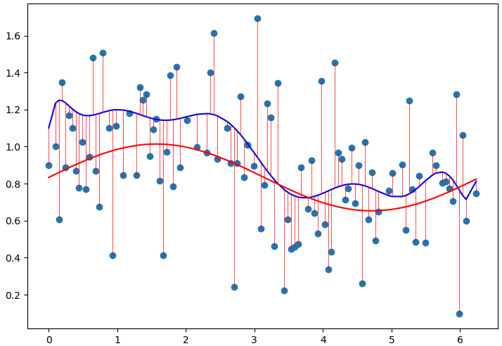
Figure 1: A polynomial of degree 11 (blue) fit to data generated following the red line.
The model with more parameters is able to fit some the noisy data slightly better. Does this necessarily mean it will perform better on new samples? No, it will usually perform worse. This is referred to as overfitting. Overfitting can be identified as the model trains. When the testing loss continues to decrease while the validation loss increases, the model is probably overfitting. It is also evident from looking at the weights.
Identifying the Cause
The goal of training is to modify the weights such that they minimize the loss function. Models with more parameters have the capacity to fit more of their training data. Given the presence of noise, this is not a good thing. A very low loss on the training set may not translate to good performance on the validation set.
Looking at weights of the trained model is a good way of detecting overfitting. From the model above, the mean of the absolute value of the weights is \(11.1\). Left unchecked, the weights will take on whatever values necessary to meet the objective function.
Penalizing Weights
The most common form of regularization is to penalize the weights from taking on a high value. That is, we define a penalty term \(E(\mathbf{w})\) that is added to the loss. The higher the weight values, the higher the total loss. Thus, optimization will also include minimizing the absolute values of the weights. A simple choice for \(E(\mathbf{w})\), especially in the context of least squares, is \(L2\) regularzation:
\[ E(\mathbf{w}) = \frac{\lambda}{2}||\mathbf{w}||^2 = \frac{\lambda}{2}\mathbf{w}^T \mathbf{w}. \]
Added to the sum-of-squares error for least squares, the final loss becomes
\[ J(\mathbf{w}) = \frac{1}{2}\sum_{i=1}^n(h(\mathbf{x}_i;\mathbf{w}) - \mathbf{y}_i)^2 + \frac{\lambda}{2} \mathbf{w}^T \mathbf{w}. \]
This choice of regularization also has the benefit of being in a form that can be minimized in closed form via the normal equations. Taking the gradient of \(J(\mathbf{w})\) above with respect to 0 and solving for \(\mathbf{w}\) yields
\[ \mathbf{w} = (\lambda I + \mathbf{X}^T\mathbf{X})^{-1}\mathbf{X}^T\mathbf{y}, \]
where \(\lambda\) is a regularization hyperparameter.
Applying this regularization term to the model above with \(\lambda=1\) yields the model shown below.
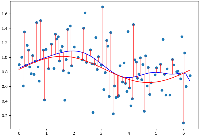
Figure 2: Least squares model fit with (L2) regularization ((lambda = 1)).
Inspecting the weights as before, we can see that the mean of the absolute values of \(\mathbf{w}\) is \(0.0938\).
Evaluating on the Testing Data
To see which model generalizes better, we set aside some samples from the original dataset to use as testing.
With regularization, the model error on the test set is \(1.8\). Without regularization, the model error on the test set is \(2.2\).
Dataset Augmentation
The same data augmentation techniques should be applied on both methods being compared. Getting a better result on a benchmark because of data augmentation does not mean the method was better suited for the task. By controlling these factors, a fair comparison can be made.
There are many forms of augmentation available for image tasks in particular. Rotating, translating, and scaling images are the most common. Additionally applying random crops can further augment the dataset.
The original dataset may only include samples of a class that have similar lighting. Color jitter is an effective way of including a broader range of hue or brightness and usually leads to a model that is robust to such changes.
It is important to make sure that the crops still contain enough information to properly classify it. Common forms of data augmentation are available through APIs like torchvision.
Early Stopping
If the validation loss begins to increase while the training loss continues to decrease, this is a clear indication that the model is beginning to overfit the training data. Stopping the model in this case is the best way to prevent this. Frameworks like PyTorch Lightning include features to checkpoing the models based on best validation loss and stop the model whenever the validation loss begins to diverge.
Dropout
Dropout is a regularization method introduced by <&srivastavaDropoutSimpleWay2014> which is motivated by ensemble methods. Ensembles of models are regularized by the fact that many different models are trained on random permutations of the dataset with varying parameters and initializations. Using an ensemble of networks is a powerful way of increasing generalization performance. However, it requires much more compute due to the fact that several models must be trained.
Training a single network with dropout approximates training several models in an ensemble. It works by randomly removing a node from the network during a forward/backward pass. The node is not truly removed. Instead, its output during the forward and backward passes is ignored via a binary mask.
When training a network with dropout, it will generally take longer for the model to converge to a solution. Intuitively, this is because a different subnetwork is being used for each pass.