Sorting in Linear Time
These are my personal notes for Chapter 8 of Introduction to Algorithms (Cormen et al. 2022). Readers should reference the book for more details when necessary.
The lecture slides for these notes are available here.
Introduction
All sorting algorithms discussed up to this point are comparison based. You may have thought, as I did, that sorting cannot be done without a comparison. If you have no way to evaluate the relative ordering of two different objects, how can you possibly arrange them in any order?
The answer will become clear shortly and is investigated through counting sort, radix sort, and bucket sort. First, Cormen et al. make it clear that sorting algorithms cannot reach linear time. As we will see, any comparison sort must make \(\Omega (n \lg n)\) comparisons in the worst case to sort \(n\) elements. This bound is motivation enough to explore a different class of sorting algorithms.
Establishing a Lower Bound on Comparison Sorts
The basis of the proof presented in Chapter 8 it to consider that all comparison sorts can be viewed as a decision tree, where each leaf represents a unique permutation of the inputs. If there are \(n\) distinct elements in the original array, then there must be \(n!\) leaves in the decision tree. Consider the figure from (Cormen et al. 2022) below.
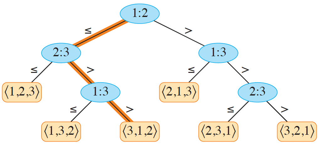
Figure 1: Decision tree for comparison sort on three elements.
In the figure above, each node compares two values as \(a:b\). If \(a \leq b\), the left path is taken. The worst case of a comparison sort can be determined by the height of the tree. A proof on the lower bound goes as follows.
Consider a binary tree of height \(h\) with \(l\) reachable leaves. Each of the \(n!\) permutations occurs as one of the leaves, so \(n! \leq l\) since there may be duplicate permutations in the leaves. A binary tree with height \(h\) has no more than \(2^h\) leaves, so \(n! \leq l \leq 2^h\). Taking the logarithm of this inequality implies that \(h \geq \lg n!\). Since \(\lg n! = \Theta(n \lg n)\), and is a lower bound on the height of the tree, then any comparison sort must make \(\Omega (n \lg n)\) comparisons.
Counting Sort
Counting sort can sort an array of integers in \(O(n+k)\) time, where \(k \geq 0\) is the largest integer in the set. It works by counting the number of elements less than or equal to each element \(x\).
def counting_sort(A, k):
    n = len(A)
    B = [0 for i in range(n)]
    C = [0 for i in range(k+1)]

    for i in range(n):
        C[A[i]] += 1
    # C[i] contains the number of elements equal to i

    for i in range(1, k):
        C[i] = C[i] + C[i-1]
    # C[i] contains the number of elements less than or equal to i

    for i in range(n - 1, -1, -1):
        B[C[A[i]]-1] = A[i]
        C[A[i]] = C[A[i]] - 1

    return B
The first two loops establish the number of elements less than or equal to \(i\) for each element \(i\). The main sticking point in understanding this algorithm is the last loop. It starts at the very end of loop, placing the last element from \(A\) into the output array \(B\) in its correct position as determined by \(C\).
Consider a simple example with \(\{2, 5, 5, 3, 4\}\). After the second loop, \(C = \{0, 0, 1, 2, 3, 5\}\). On the first iteration of the last loop, \(A[4] = 4\) is used as the index into \(C\), which yields \(3\) since the value \(4\) is greater than or equal to \(3\) elements in the original array. It is then placed in the correct spot \(B[3-1] = 4\).
Another example is shown in figure 8.2 from (Cormen et al. 2022).
Radix Sort
Dating back to 1887 by Herman Hollerith’s work on tabulating machines, this algorithm places numbers in one of \(k\) bins based on their radix, or the number of unique digits. It was used for sorting punch cards via multi-column sorting. It works by iteratively sorting a series of inputs based on a column starting with the least-significant digit. An example is shown below.
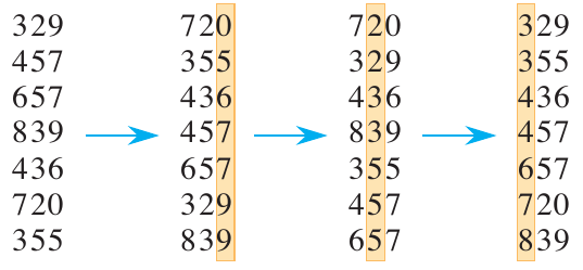
Figure 2: Radix sort in action (Cormen et al. 2022).
In the figure above, the items are first sorted based on the least significant digits. By the end of the process, the data is numerically sorted in ascending order. The algorithm can be written simply:
def radix_sort(A, d):
    for i in range(d):
        A = counting_sort(A, len(A), 9)
    return A
Counting sort is the typical sorting algorithm that is used to sort the digits in each column. In fact, any stable sorting algorithm can be used in place of counting sort.
Analysis
We know that counting sort is \(\Theta(n + k)\), and that radix sort calls it \(d\) times. Therefore, the time complexity of radix sort is \(\Theta(d(n + k))\). If \(k = O(n)\), then the time complexity is \(\Theta(dn)\).
Complex Keys
What if the data is not just a single integer, but a complex key or series of keys? The keys themselves can be broken up into digits. Consider a 32-bit word. If we want to sort \(n\) of these words, and we have \(b = 32\) bits per word, we can break the words into \(r=8\) bit digits. This yields \(d = \lceil b / r \rceil = 4\) digits. The largest value for each digit is then \(k = 2^r - 1 = 255\). Plugging these values into the analysis from above yields $Θ((b/r)(n + 2^r)).$
What is the best choice of \(r\)? Consider what happens for different values of \(r\). As \(r\) increases, \(2^r\) increases. As it decreases, \(\frac{b}{r}\) increases. The best choice depends on whether \(b < \lfloor \lg n \rfloor\). If \(b < \lfloor \lg n \rfloor\), then \(r \leq b\) implies \((n + 2^r) = \Theta(n)\) since \(2^{\lg n} = n\). If \(b \geq \lfloor \lg n \rfloor\), then we should choose \(r \approx \lg n\). This would yield \(\Theta((b / \lg n)(n + n)) = \Theta(bn / \lg n)\).
You should spend some time to think about the choices for \(r\). Specifically, what will happen to the time complexity as \(r\) increases above \(\lg n\)? What about as \(r\) decreases below \(\lg n\)?
Example: Sorting words
Use radix sort to sort the following list of names: “Beethoven”, “Bach”, “Mozart”, “Chopin”, “Liszt”, “Schubert”, “Haydn”, “Brahms”, “Wagner”, “Tchaikovsky”. First, we need to figure out how to encode the names as integers. If we convert the input to lowercase, we only have to deal with \(k=26\) unique characters. This only requires 5 bits. Since each name has varying length, we can use a sentinel value of 0 to pad the shorter names. That is, 0 represents a padding character and the alphabet starts at 1. The names are then encoded as follows:
| Original Name | Encoded Name |
|---|---|
| Beethoven | [2, 5, 5, 20, 8, 15, 22, 5, 14, 0, 0] |
| Bach | [2, 1, 3, 8, 0, 0, 0, 0, 0, 0, 0] |
| Mozart | [13, 15, 26, 1, 18, 20, 0, 0, 0, 0, 0] |
| Chopin | [3, 8, 15, 16, 9, 14, 0, 0, 0, 0, 0] |
| Liszt | [12, 9, 19, 26, 20, 0, 0, 0, 0, 0, 0] |
| Schubert | [19, 3, 8, 21, 2, 5, 18, 20, 0, 0, 0] |
| Haydn | [8, 1, 25, 4, 14, 0, 0, 0, 0, 0, 0] |
| Brahms | [2, 18, 1, 8, 13, 19, 0, 0, 0, 0, 0] |
| Wagner | [23, 1, 7, 14, 5, 18, 0, 0, 0, 0, 0] |
| Tchaikovsky | [20, 3, 8, 1, 9, 11, 15, 22, 19, 11, 25] |
No changes will be made for the first 2 iterations of the sort. The third iteration will yield the following:
| Original Name | Encoded Name |
|---|---|
| Bach | [2, 1, 3, 8, 0, 0, 0, 0, 0, 0, 0] |
| Mozart | [13, 15, 26, 1, 18, 20, 0, 0, 0, 0, 0] |
| Chopin | [3, 8, 15, 16, 9, 14, 0, 0, 0, 0, 0] |
| Liszt | [12, 9, 19, 26, 20, 0, 0, 0, 0, 0, 0] |
| Schubert | [19, 3, 8, 21, 2, 5, 18, 20, 0, 0, 0] |
| Haydn | [8, 1, 25, 4, 14, 0, 0, 0, 0, 0, 0] |
| Brahms | [2, 18, 1, 8, 13, 19, 0, 0, 0, 0, 0] |
| Wagner | [23, 1, 7, 14, 5, 18, 0, 0, 0, 0, 0] |
| Beethoven | [2, 5, 5, 20, 8, 15, 22, 5, 14, 0, 0] |
| Tchaikovsky | [20, 3, 8, 1, 9, 11, 15, 22, 19, 11, 25] |
Iteration 3
| Original Name | Encoded Name |
|---|---|
| Bach | [2, 1, 3, 8, 0, 0, 0, 0, 0, 0, 0] |
| Mozart | [13, 15, 26, 1, 18, 20, 0, 0, 0, 0, 0] |
| Chopin | [3, 8, 15, 16, 9, 14, 0, 0, 0, 0, 0] |
| Liszt | [12, 9, 19, 26, 20, 0, 0, 0, 0, 0, 0] |
| Haydn | [8, 1, 25, 4, 14, 0, 0, 0, 0, 0, 0] |
| Brahms | [2, 18, 1, 8, 13, 19, 0, 0, 0, 0, 0] |
| Wagner | [23, 1, 7, 14, 5, 18, 0, 0, 0, 0, 0] |
| Schubert | [19, 3, 8, 21, 2, 5, 18, 20, 0, 0, 0] |
| Beethoven | [2, 5, 5, 20, 8, 15, 22, 5, 14, 0, 0] |
| Tchaikovsky | [20, 3, 8, 1, 9, 11, 15, 22, 19, 11, 25] |
Iteration 4
| Original Name | Encoded Name |
|---|---|
| Bach | [2, 1, 3, 8, 0, 0, 0, 0, 0, 0, 0] |
| Liszt | [12, 9, 19, 26, 20, 0, 0, 0, 0, 0, 0] |
| Haydn | [8, 1, 25, 4, 14, 0, 0, 0, 0, 0, 0] |
| Schubert | [19, 3, 8, 21, 2, 5, 18, 20, 0, 0, 0] |
| Tchaikovsky | [20, 3, 8, 1, 9, 11, 15, 22, 19, 11, 25] |
| Chopin | [3, 8, 15, 16, 9, 14, 0, 0, 0, 0, 0] |
| Beethoven | [2, 5, 5, 20, 8, 15, 22, 5, 14, 0, 0] |
| Wagner | [23, 1, 7, 14, 5, 18, 0, 0, 0, 0, 0] |
| Brahms | [2, 18, 1, 8, 13, 19, 0, 0, 0, 0, 0] |
| Mozart | [13, 15, 26, 1, 18, 20, 0, 0, 0, 0, 0] |
Iteration 5
| Original Name | Encoded Name |
|---|---|
| Bach | [2, 1, 3, 8, 0, 0, 0, 0, 0, 0, 0] |
| Schubert | [19, 3, 8, 21, 2, 5, 18, 20, 0, 0, 0] |
| Wagner | [23, 1, 7, 14, 5, 18, 0, 0, 0, 0, 0] |
| Beethoven | [2, 5, 5, 20, 8, 15, 22, 5, 14, 0, 0] |
| Tchaikovsky | [20, 3, 8, 1, 9, 11, 15, 22, 19, 11, 25] |
| Chopin | [3, 8, 15, 16, 9, 14, 0, 0, 0, 0, 0] |
| Brahms | [2, 18, 1, 8, 13, 19, 0, 0, 0, 0, 0] |
| Haydn | [8, 1, 25, 4, 14, 0, 0, 0, 0, 0, 0] |
| Mozart | [13, 15, 26, 1, 18, 20, 0, 0, 0, 0, 0] |
| Liszt | [12, 9, 19, 26, 20, 0, 0, 0, 0, 0, 0] |
Iteration 6
| Original Name | Encoded Name |
|---|---|
| Tchaikovsky | [20, 3, 8, 1, 9, 11, 15, 22, 19, 11, 25] |
| Mozart | [13, 15, 26, 1, 18, 20, 0, 0, 0, 0, 0] |
| Haydn | [8, 1, 25, 4, 14, 0, 0, 0, 0, 0, 0] |
| Bach | [2, 1, 3, 8, 0, 0, 0, 0, 0, 0, 0] |
| Brahms | [2, 18, 1, 8, 13, 19, 0, 0, 0, 0, 0] |
| Wagner | [23, 1, 7, 14, 5, 18, 0, 0, 0, 0, 0] |
| Chopin | [3, 8, 15, 16, 9, 14, 0, 0, 0, 0, 0] |
| Beethoven | [2, 5, 5, 20, 8, 15, 22, 5, 14, 0, 0] |
| Schubert | [19, 3, 8, 21, 2, 5, 18, 20, 0, 0, 0] |
| Liszt | [12, 9, 19, 26, 20, 0, 0, 0, 0, 0, 0] |
Iteration 7
| Original Name | Encoded Name |
|---|---|
| Brahms | [2, 18, 1, 8, 13, 19, 0, 0, 0, 0, 0] |
| Bach | [2, 1, 3, 8, 0, 0, 0, 0, 0, 0, 0] |
| Beethoven | [2, 5, 5, 20, 8, 15, 22, 5, 14, 0, 0] |
| Wagner | [23, 1, 7, 14, 5, 18, 0, 0, 0, 0, 0] |
| Tchaikovsky | [20, 3, 8, 1, 9, 11, 15, 22, 19, 11, 25] |
| Schubert | [19, 3, 8, 21, 2, 5, 18, 20, 0, 0, 0] |
| Chopin | [3, 8, 15, 16, 9, 14, 0, 0, 0, 0, 0] |
| Liszt | [12, 9, 19, 26, 20, 0, 0, 0, 0, 0, 0] |
| Haydn | [8, 1, 25, 4, 14, 0, 0, 0, 0, 0, 0] |
| Mozart | [13, 15, 26, 1, 18, 20, 0, 0, 0, 0, 0] |
Iteration 8
| Original Name | Encoded Name |
|---|---|
| Bach | [2, 1, 3, 8, 0, 0, 0, 0, 0, 0, 0] |
| Haydn | [8, 1, 25, 4, 14, 0, 0, 0, 0, 0, 0] |
| Wagner | [23, 1, 7, 14, 5, 18, 0, 0, 0, 0, 0] |
| Tchaikovsky | [20, 3, 8, 1, 9, 11, 15, 22, 19, 11, 25] |
| Schubert | [19, 3, 8, 21, 2, 5, 18, 20, 0, 0, 0] |
| Beethoven | [2, 5, 5, 20, 8, 15, 22, 5, 14, 0, 0] |
| Chopin | [3, 8, 15, 16, 9, 14, 0, 0, 0, 0, 0] |
| Liszt | [12, 9, 19, 26, 20, 0, 0, 0, 0, 0, 0] |
| Mozart | [13, 15, 26, 1, 18, 20, 0, 0, 0, 0, 0] |
| Brahms | [2, 18, 1, 8, 13, 19, 0, 0, 0, 0, 0] |
Iteration 9
| Original Name | Encoded Name |
|---|---|
| Bach | [2, 1, 3, 8, 0, 0, 0, 0, 0, 0, 0] |
| Beethoven | [2, 5, 5, 20, 8, 15, 22, 5, 14, 0, 0] |
| Brahms | [2, 18, 1, 8, 13, 19, 0, 0, 0, 0, 0] |
| Chopin | [3, 8, 15, 16, 9, 14, 0, 0, 0, 0, 0] |
| Haydn | [8, 1, 25, 4, 14, 0, 0, 0, 0, 0, 0] |
| Liszt | [12, 9, 19, 26, 20, 0, 0, 0, 0, 0, 0] |
| Mozart | [13, 15, 26, 1, 18, 20, 0, 0, 0, 0, 0] |
| Schubert | [19, 3, 8, 21, 2, 5, 18, 20, 0, 0, 0] |
| Tchaikovsky | [20, 3, 8, 1, 9, 11, 15, 22, 19, 11, 25] |
| Wagner | [23, 1, 7, 14, 5, 18, 0, 0, 0, 0, 0] |
Bucket Sort
The final sorting algorithm in Chapter 8 is bucket sort (Cormen et al. 2022). As the name suggests, bucket sort distributes the input into a number of distinct buckets based on the input value. The key here is the assumption that the data is uniformly distributed. If the data were not uniformly distributed, then more elements would be concentrated. The uniformity ensures that a relatively equal number of data points are placed in each bucket. This is also a convenient assumption to have for a parallelized implementation.
The algorithm works by placing values into a bucket based on their most significant digits. Once the values are assigned, then a simple sort, like insertion sort, is used to sort the values within each bucket. Once sorted, the buckets are concatenated together to produce the final output. Under the assumption of uniformity, each bucket will contain no more than \(1/n\) of the total elements. This implies that each call to insertion_sort will take \(O(1)\) time.

Figure 3: Bucket sort in action (Cormen et al. 2022).
def bucket_sort(A):
    n = len(A)
    B = [[] for i in range(n)]
    for i in range(n):
        B[int(n * A[i])].append(A[i])
    for i in range(n):
        insertion_sort(B[i])
    return B
Analysis
Initializing the array and placing each item into a bucket takes \(\Theta(n)\) time. The call to each insertion sort is \(O(n^2)\). Therefore, the recurrence is given as
\[ T(n) = \Theta(n) + \sum_{i=0}^{n-1} O(n_i^2). \]
The key is to determine the expected value \(E[n_i^2]\). We will frame the problem as a binomial distribution, where a success occurs when an element goes into bucket \(i\).
- \(p\) is the probability of success: \(p = \frac{1}{n}\).
- \(q\) is the probability of failure: \(q = 1 - \frac{1}{n}\).
Under a binomial distribution, we have that \(E[n_i] = np = n(1/n) = 1\) and \(\text{Var}[n_i] = npq = 1 - 1/n\), where \(p = 1/n\) and \(q = 1 - 1/n\). The expected value is then
\[ E[n_i^2] = \text{Var}[n_i] + E[n_i]^2 = 1 - 1/n + 1 = 2 - 1/n. \]
This gives way to the fact that \(E[T(n)] = \Theta(n) + \sum_{i=0}^{n-1} O(2 - 1/n) = \Theta(n) + O(n) = \Theta(n)\).
Questions and Exercises
- Come up with applications of counting sort when \(k = O(n)\).
- Paul wants to use radix sort to sort \(2^{16}\) 32-bit numbers. What is the best value of \(r\) to use? How many calls to a stable sort will be made?
- In what ways does radix sort differ from quicksort? When is one better than the other?